Various techniques to visualize and understand CNNs. Activations: Nearest neighbors, PCA, t-SNE, saliency, occlusion, backpropagation. Gradients: Saliency maps, class visualization, fooling images, feature inversion. Fun: DeepDream, texture synthesis, style transfer.

@Credits: EECS 498.007 | Video Lecture: UM-CV 5 Neural Networks

Personal work for the assignments of the course: github repo.

Notice on Usage and Attribution

These are personal class notes based on the University of Michigan EECS 498.008 / 598.008 course. They are intended solely for personal learning and academic discussion, with no commercial use.

For detailed information, please refer to the complete notice at the end of this document

Visualizing layers

First layer: Visualize filters

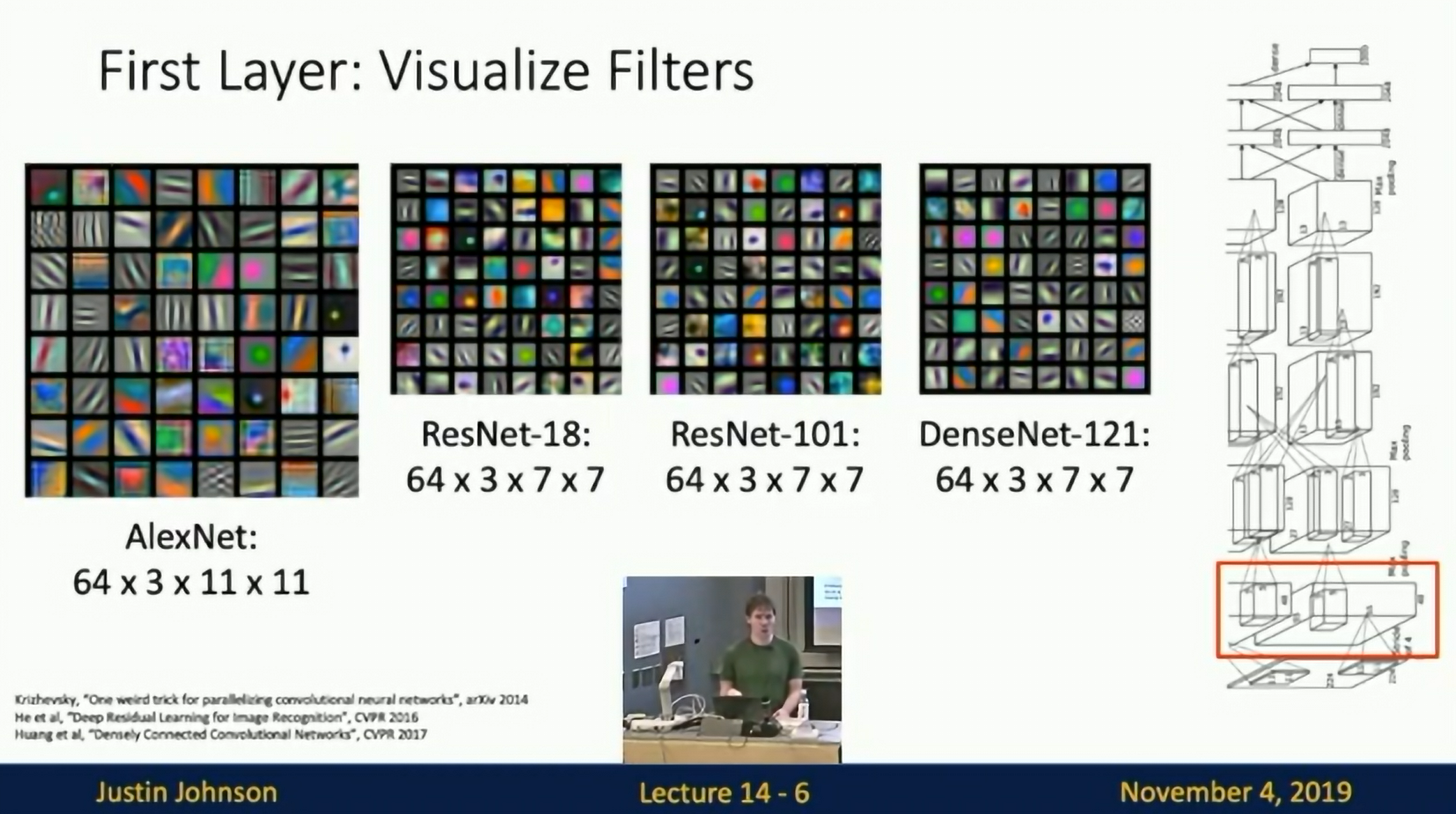
Fig: Convolutional filters on the first layer

One weird trick for parallelizing convolutional neural networks

"Template matching". Idea: inner product between filter and image region. Visualizing filters can give us some insight into what the network is looking for. Recall that Mammalian visual cortex has simple cells and complex cells. Simple cells are edge detectors, complex cells are invariant to position.

Higher Layers

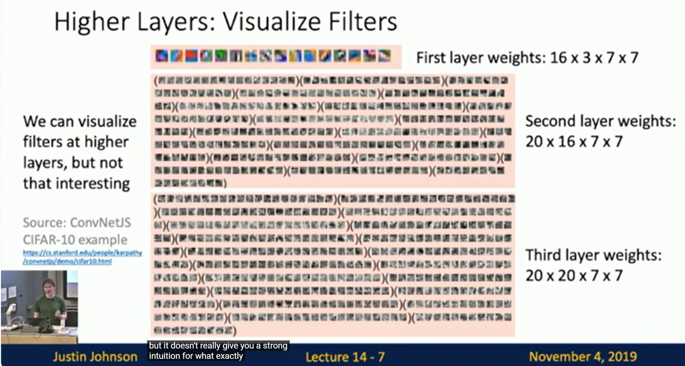
Figs: Filters on higher layers

Intermediate convolutional layers are more difficult to interpret.

Last Layer

Run the network on an image and visualize the activations of the last layer.

Nearest Neighbors

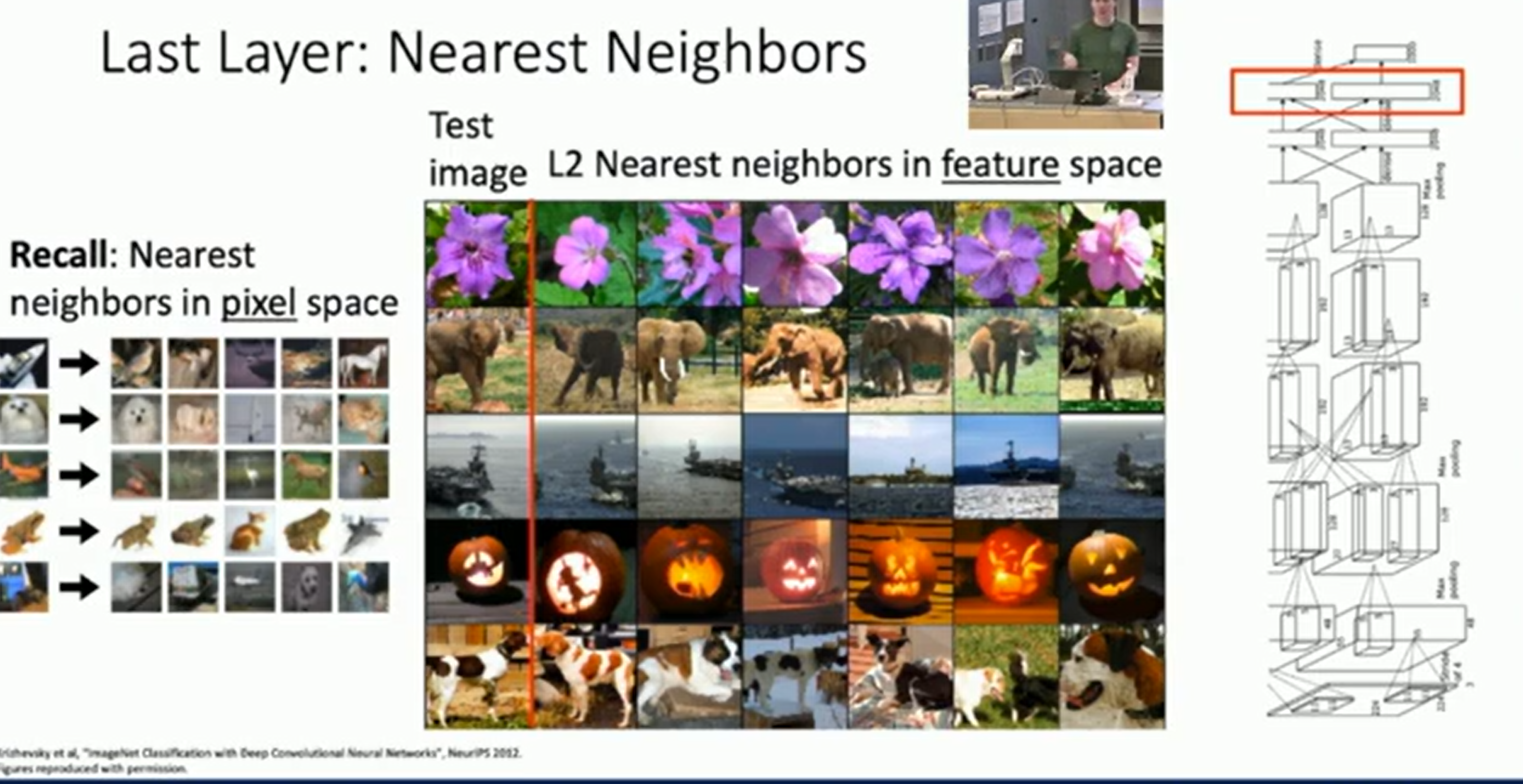
Fig: Nearest Neighbors

All of the nearest neighbors are of the same class. This is a good sign that the low-level pixel content are ignored and the network is focusing on the high-level content.

Dimensionality Reduction: PCA/t-SNE

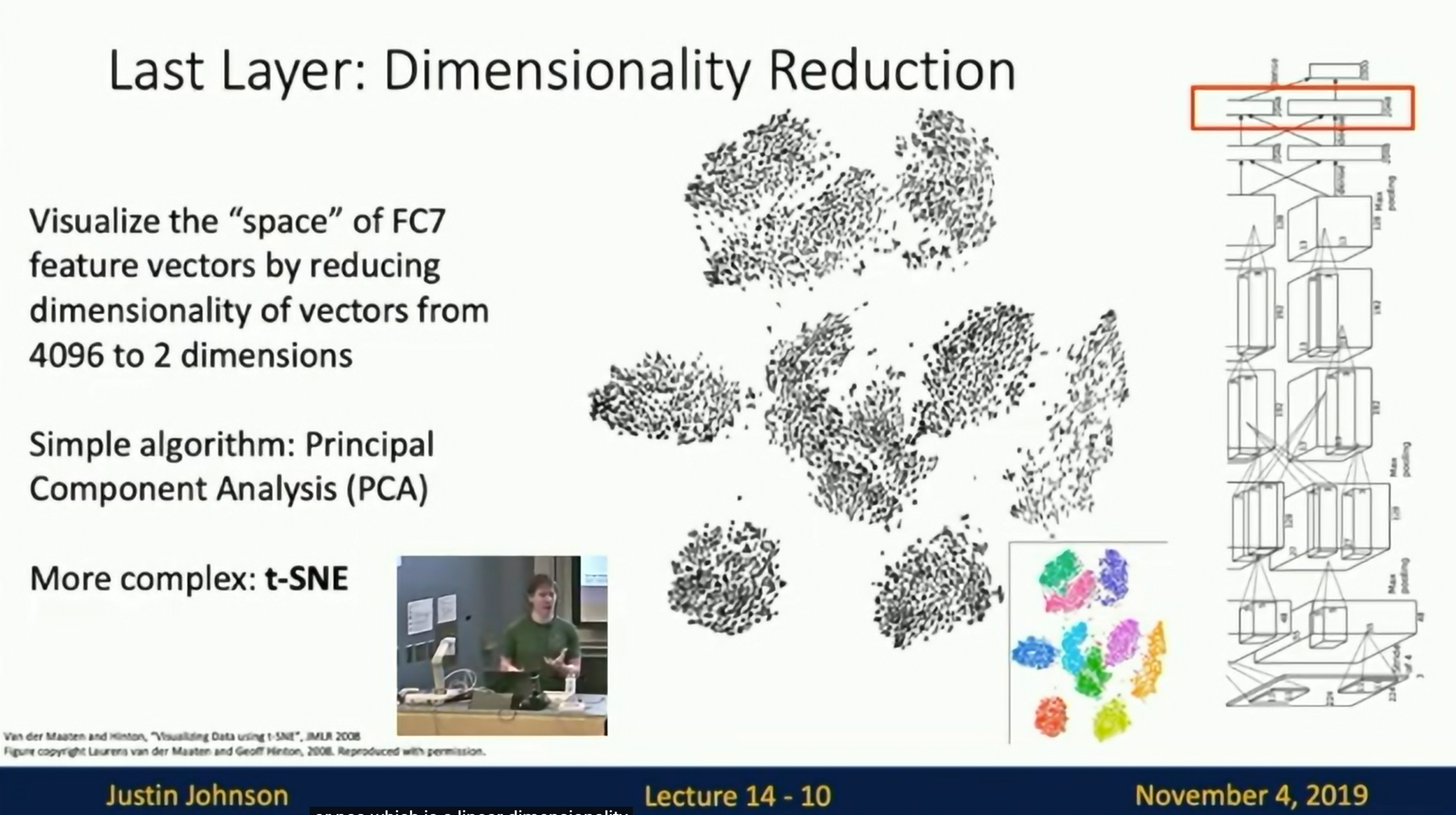
Fig: Dimensionality Reduction: PCA

t-SNE is a more complex method that tries to preserve the local structure of the data.

The ten clusters are correspond to the ten classes of MNIST.

See also high-resolution version. (Recommended, really interesting)

Visualizing Activations

Idea: Given an image, visualize the activations of the network at each layer. This gives a sense of what the neurons might be responding to.

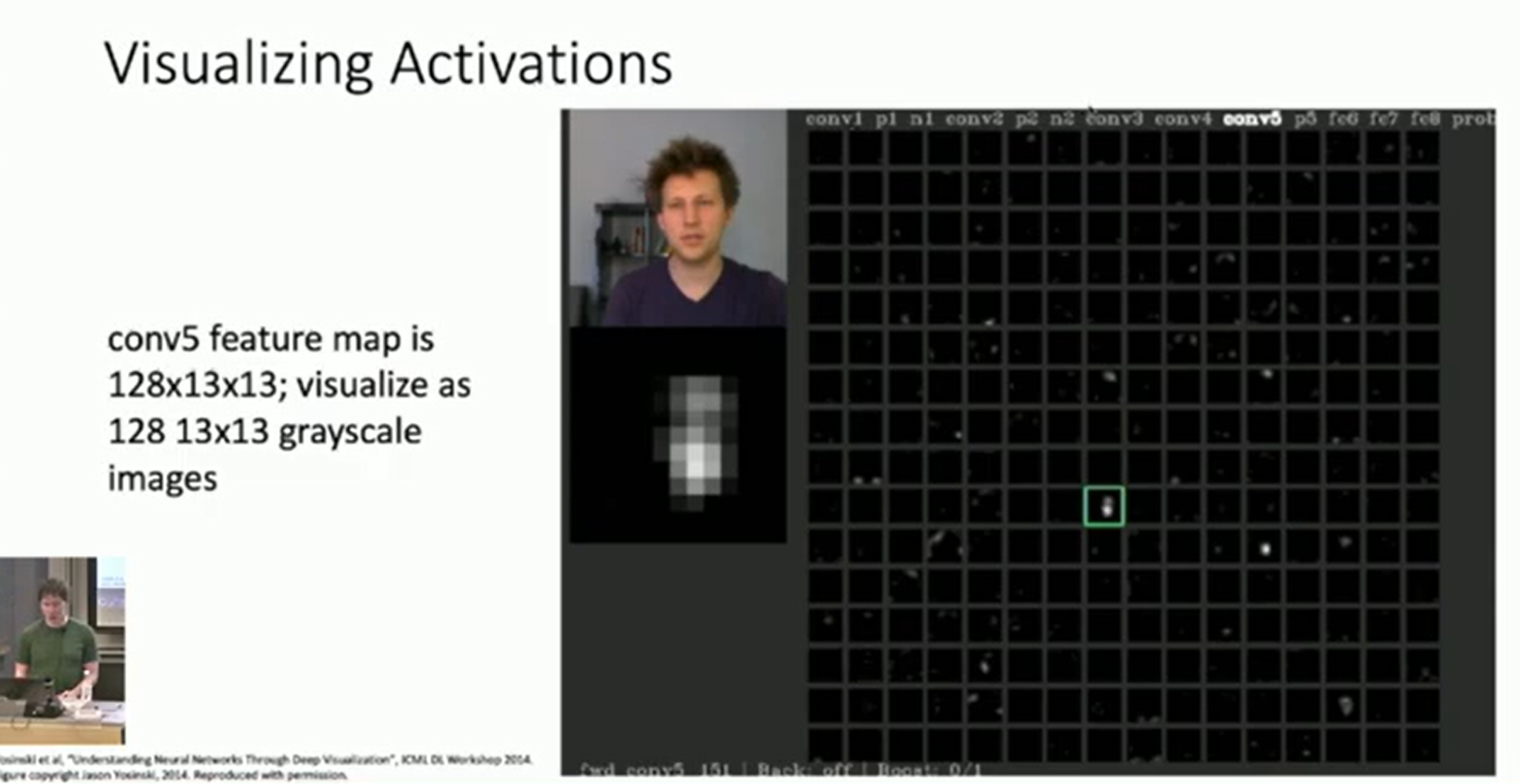
Fig: Visualizing Activations

Why are there so many zeros ? Because of the ReLU activation function. The way to squash the image might also have an effect on the visualization.

Maximally Activating Patches

Run the model on all images, and for a given neuron, find the images that maximally activate that neuron.

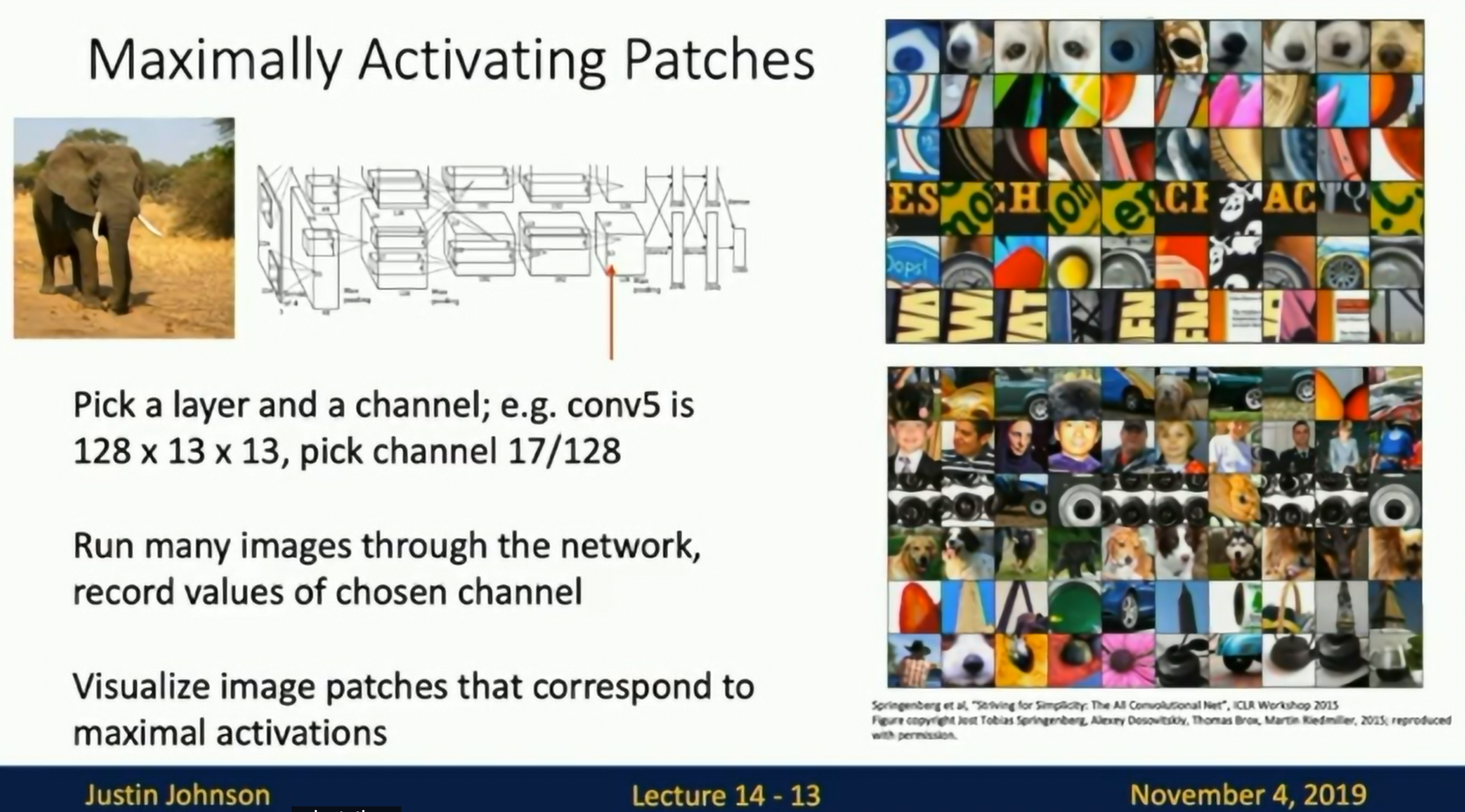
Fig: Maximally Activating Patches

Saliency via Occlusion

Pass the masked image through the network and see how the output changes.

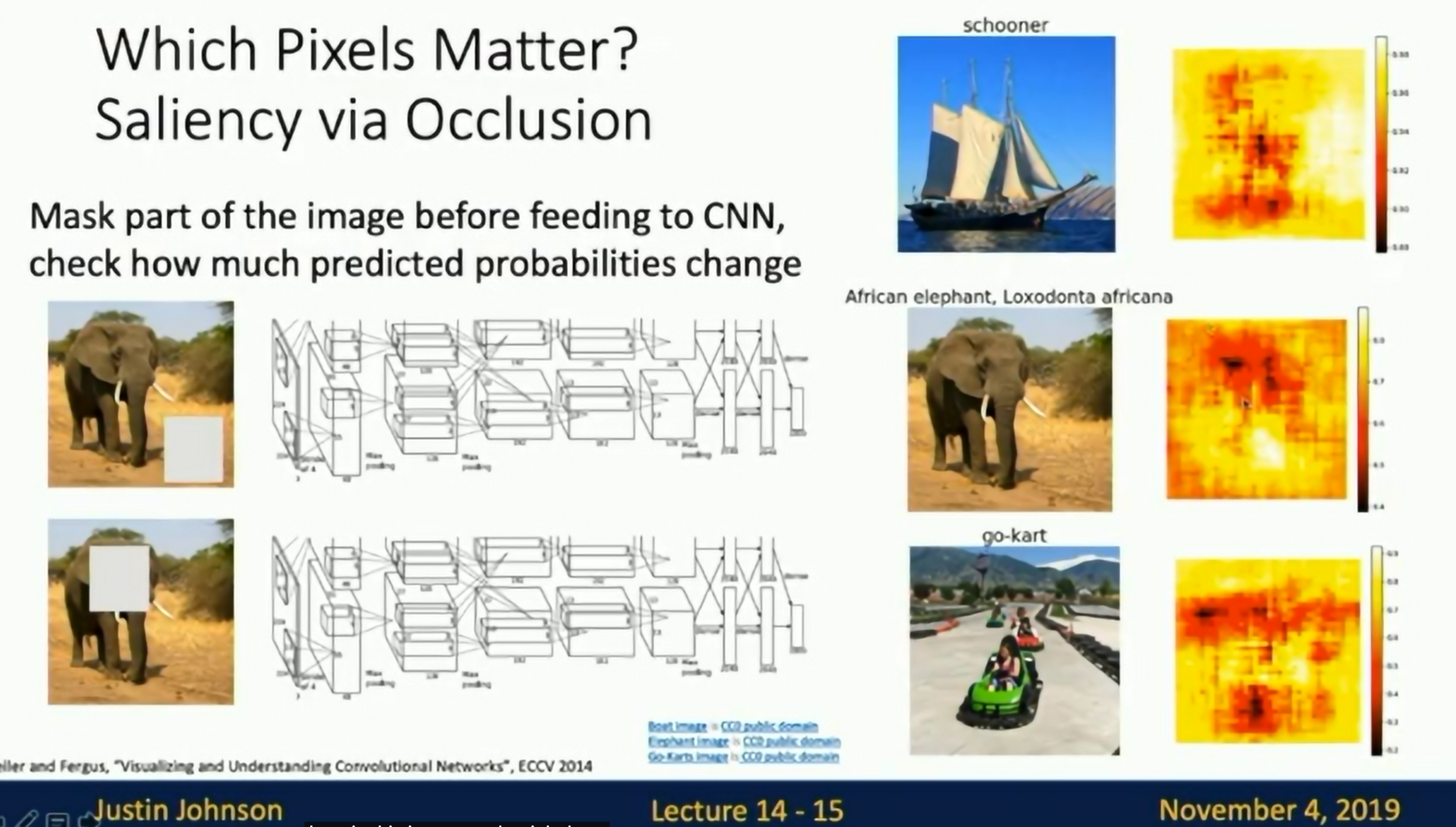
Fig: Saliency via Occlusion

Computationally expensive.

Saliency via backpropagation

Compute the gradient of the output with respect to the input.

This represents if we change the pixels a little bit, how much would it affect the score at the end.

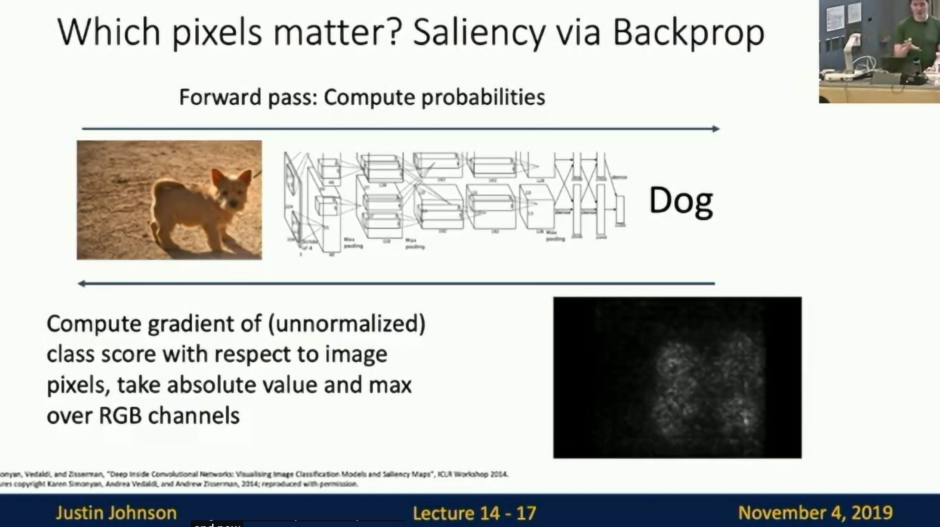
Fig: Saliency via backpropagation

(Most real examples do not look this good)

Saliency Maps: Segmentation without supervision

We can use classification models to generate segmentation masks.

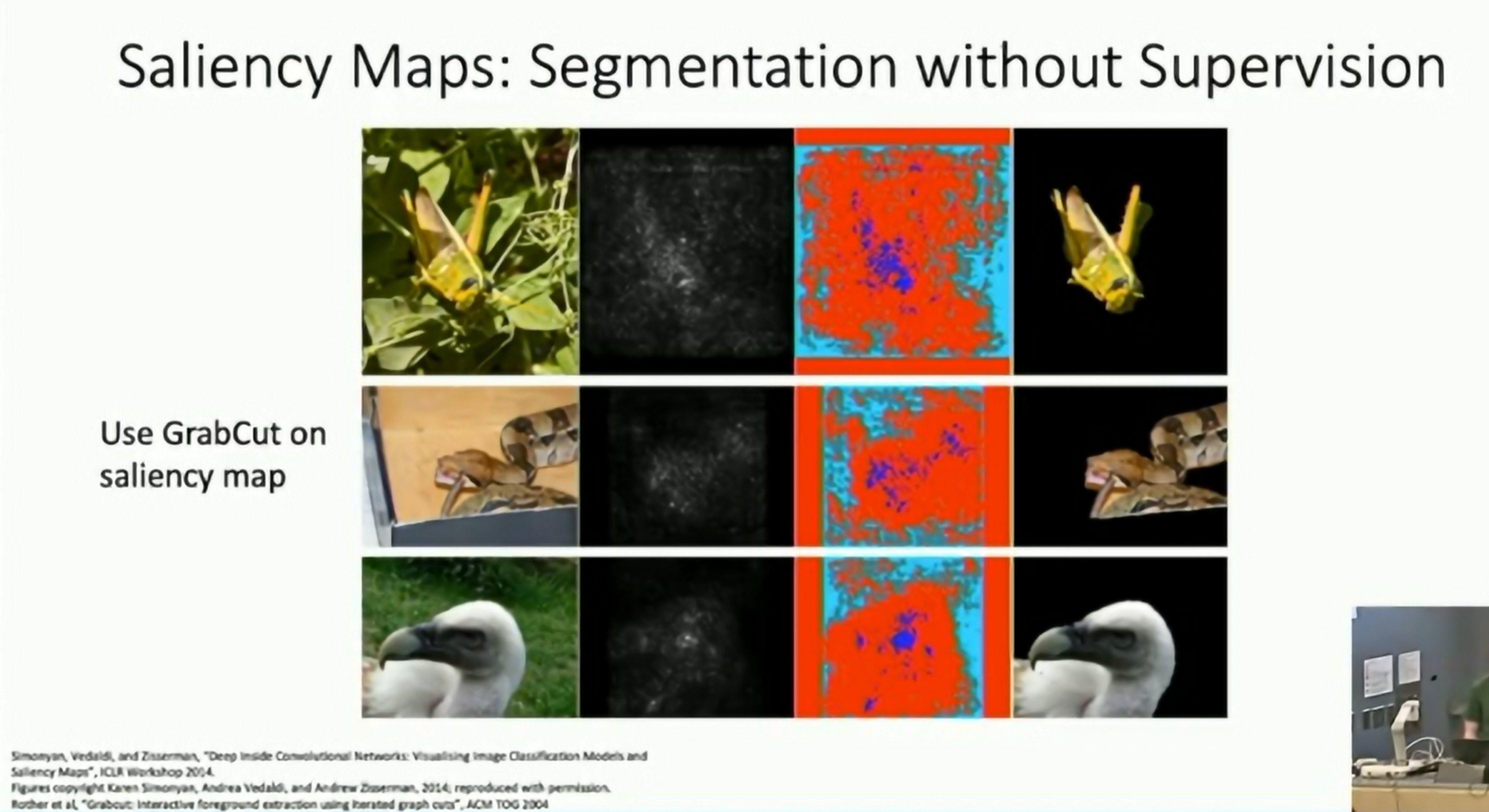
Fig: Saliency Maps: Segmentation without supervision

Gradient information for intermediate layers

Intermediate Features via (guided) backpropagation. The idea is similar to saliency via backpropagation, but if we do it directly, the results will be noisy. Instead, we use "guided backpropagation" to get cleaner results.

In forward pass, negative values are clamp to zero, and the gradients of the negative values are set to zero. In the backward pass, we also add a ReLU to the gradients, so that only positive gradients are propagated back. (Heuristic that works in practice)

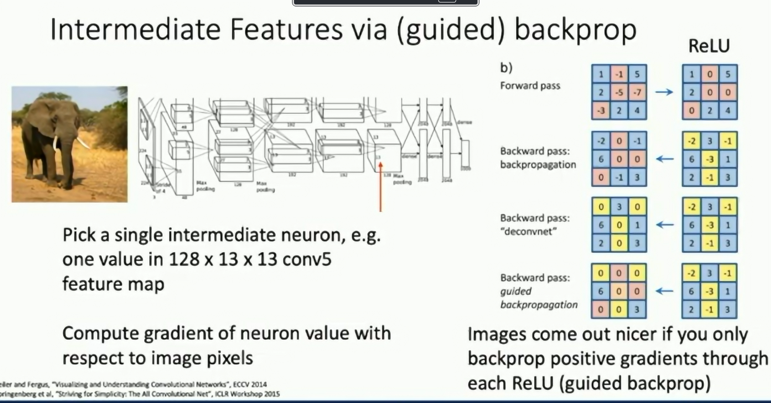
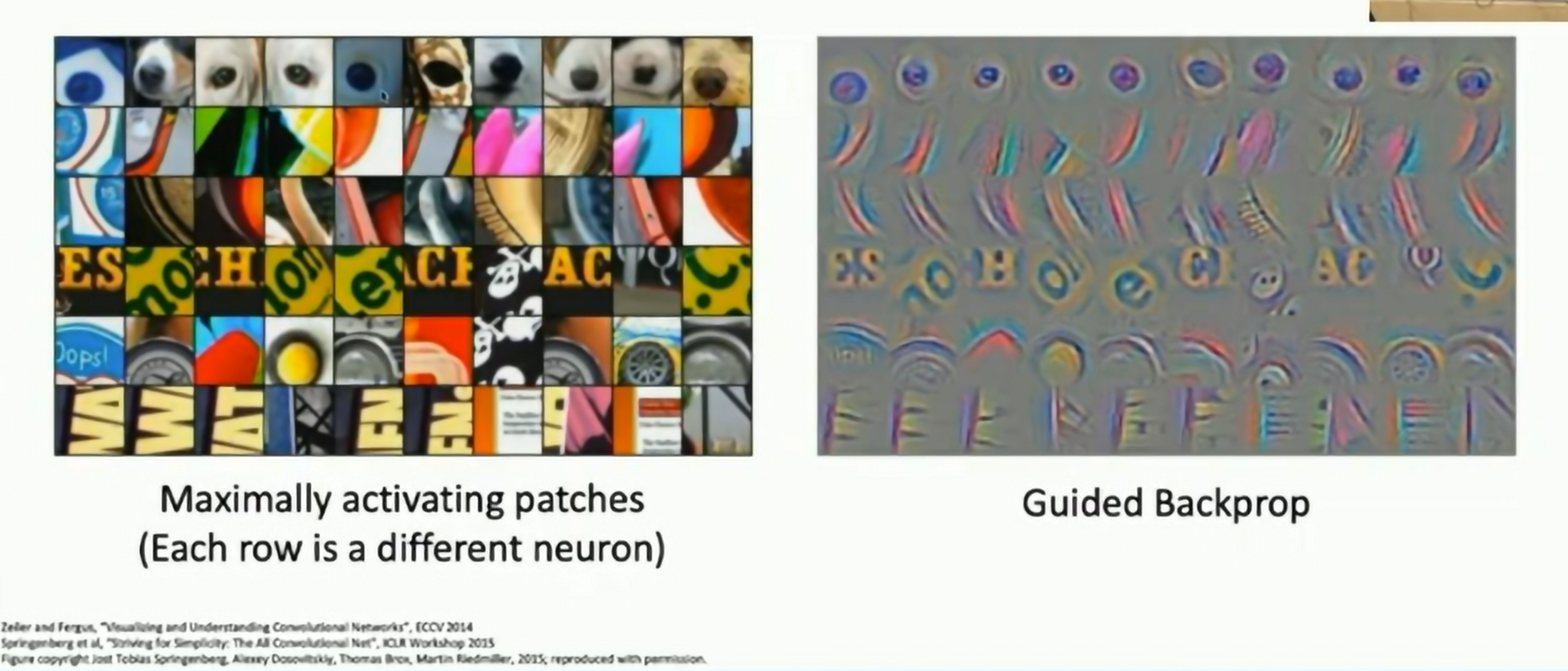
Fig: Guided Backpropagation

Gradient Ascent

Generate an image that maximizes the activation of a neuron (using gradient ascent).

Initialize original image to zero, and then update the image to maximize the activation of a neuron.

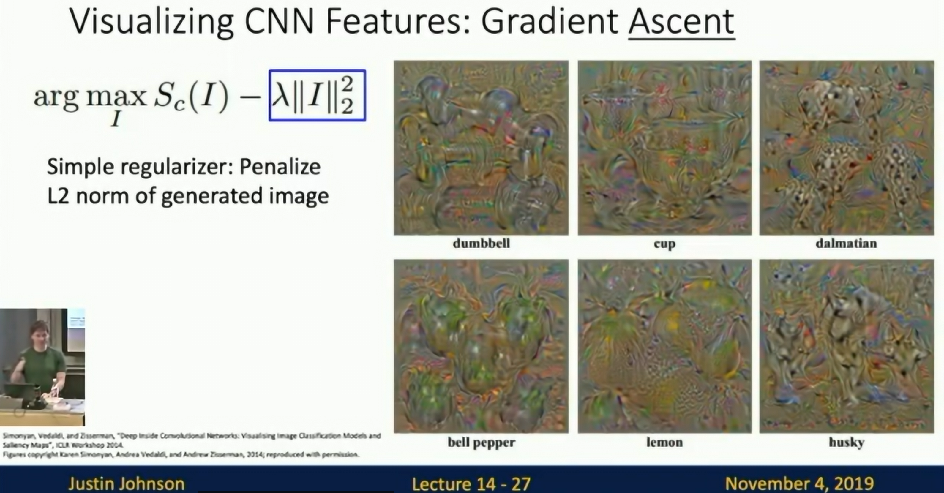
Fig: Gradient Ascent

Using other regularizers:

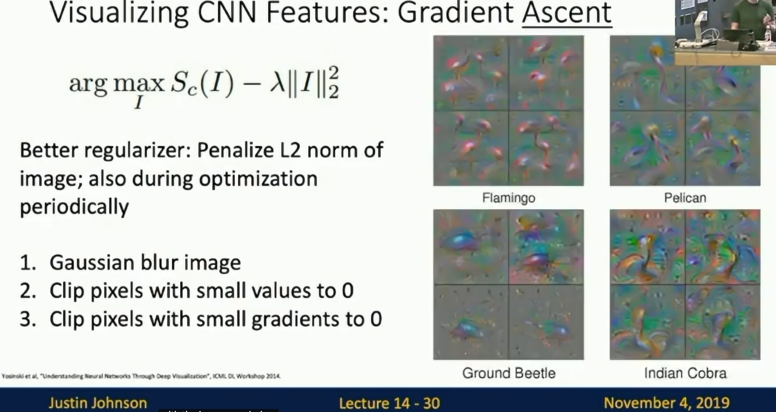
Fig: Gradient Ascent

Use the same approach to visualize intermediate features:

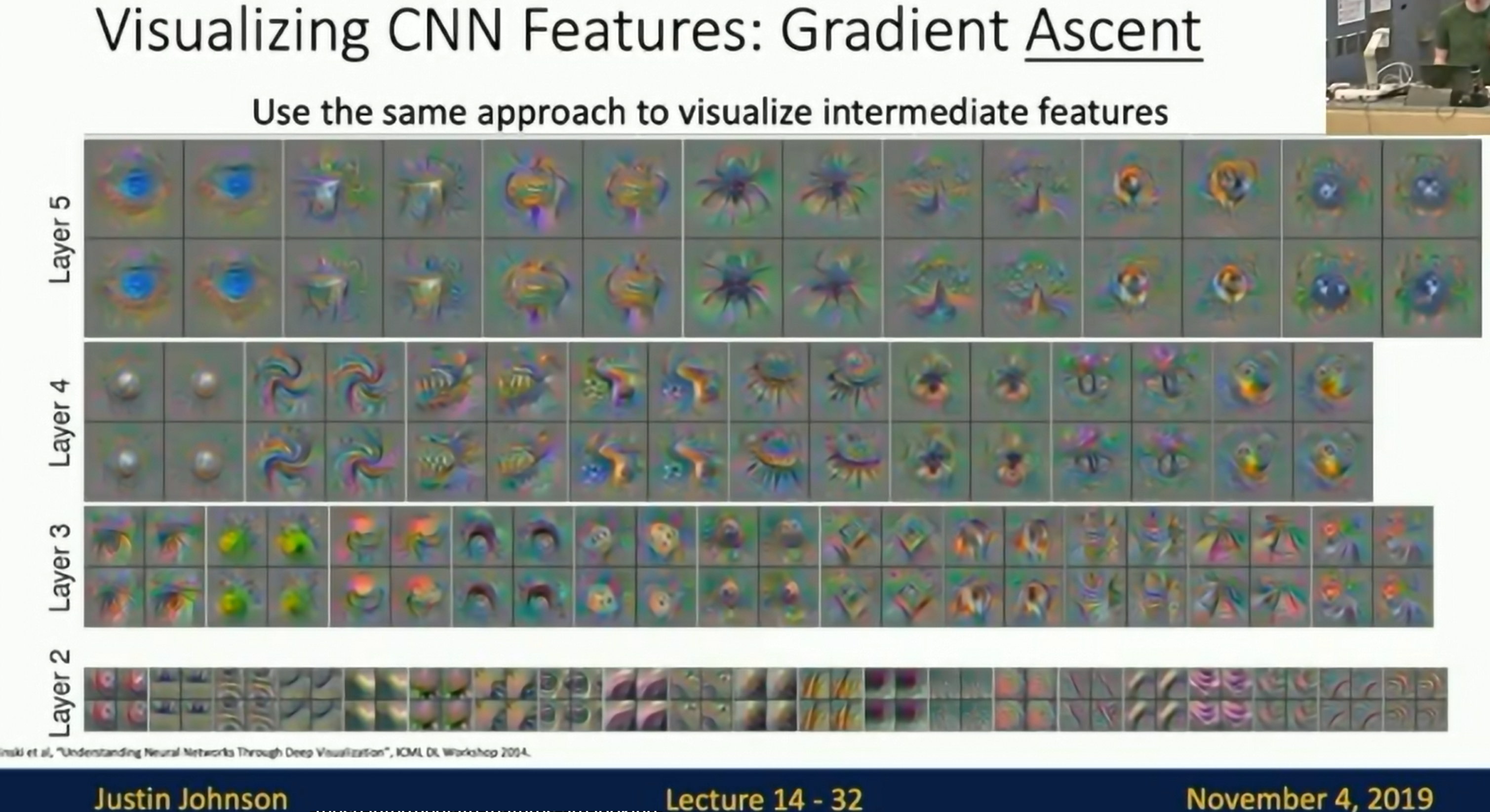
Fig: Gradient Ascent

Adversarial Examples

If we do not add regularizers, we can generate adversarial examples that looks like noise but can fool the network.

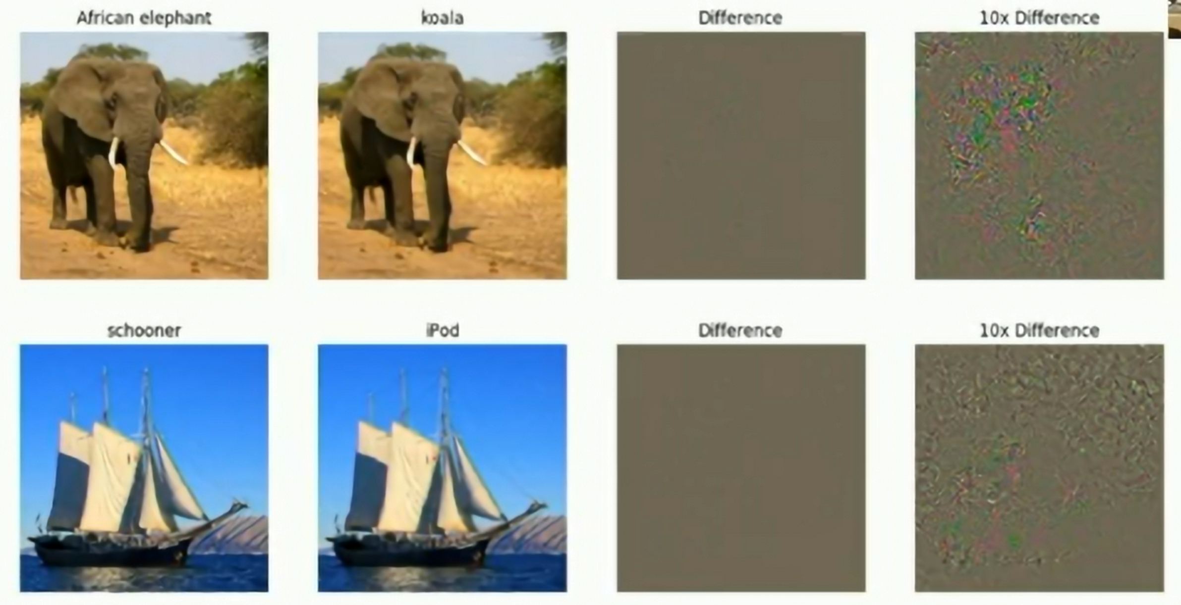
Fig: Adversarial Examples

Feature Inversion

• Feature Inversion: Given a feature vector, by minimizing the difference between the new input feature and the original feature, reconstruct an input data (such as an image).
• Gradient Ascent: By adjusting the input data, maximize the activation value of a specific neuron, and generate an input that maximizes the activation value of the neuron.

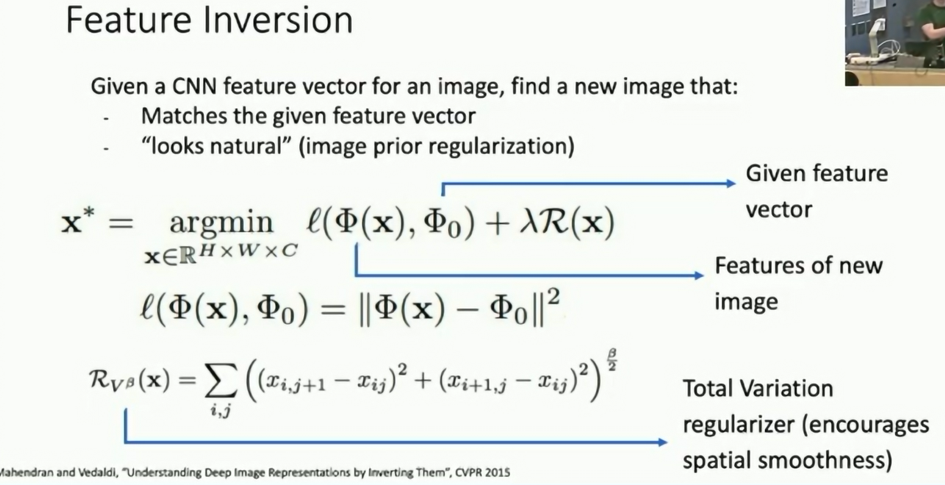
Fig: Feature Inversion

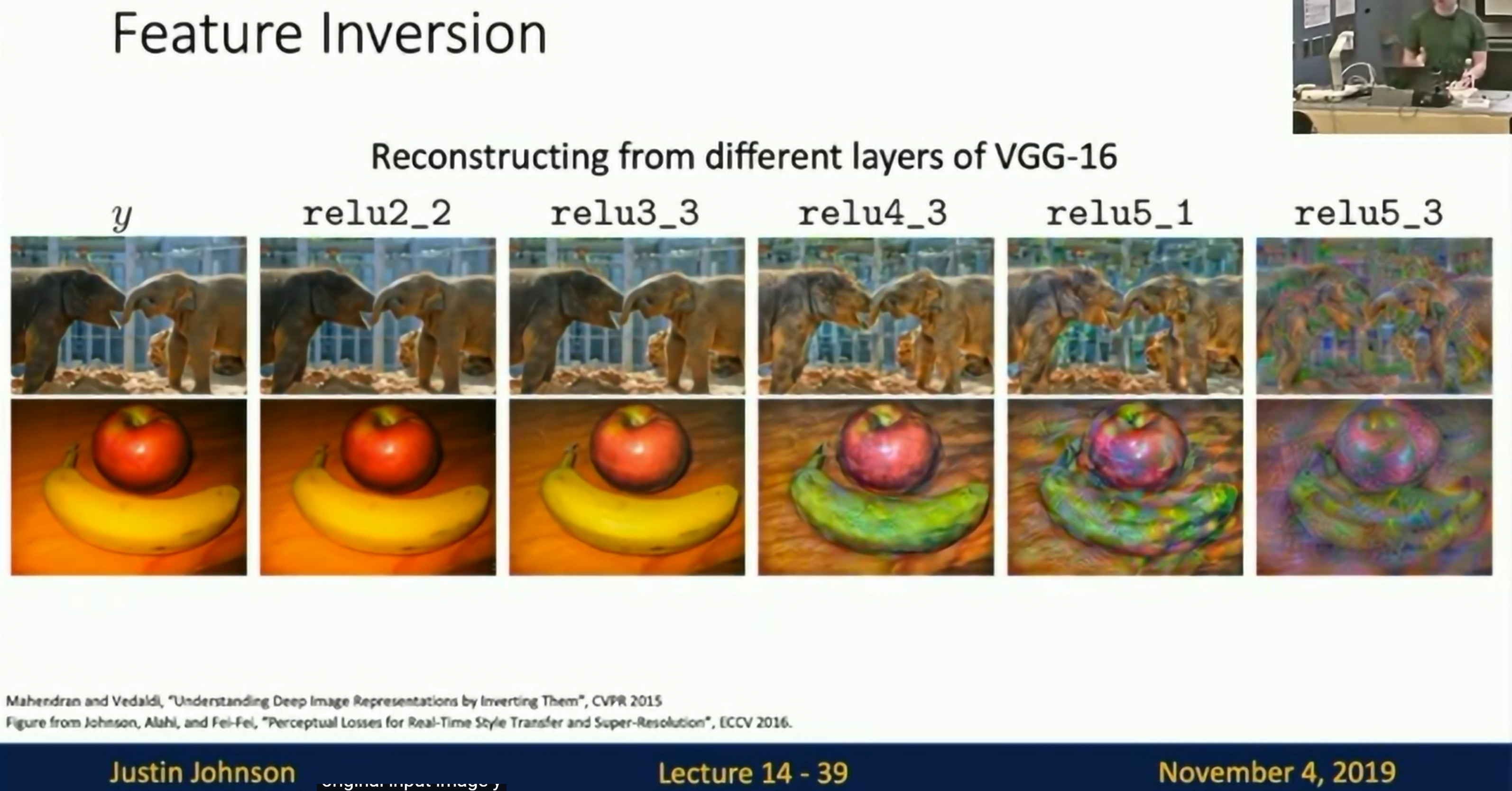
Fig: Feature Inversion

As we go up through the network, the overall structure is preserved but the details are lost. e.g. textures

DeepDream: Amplifying existing features

Take an existing image and amplify the features that are already present in the image.

Idea: Start with an image, run it through the network, and then update the image to maximize the activation of a neuron.

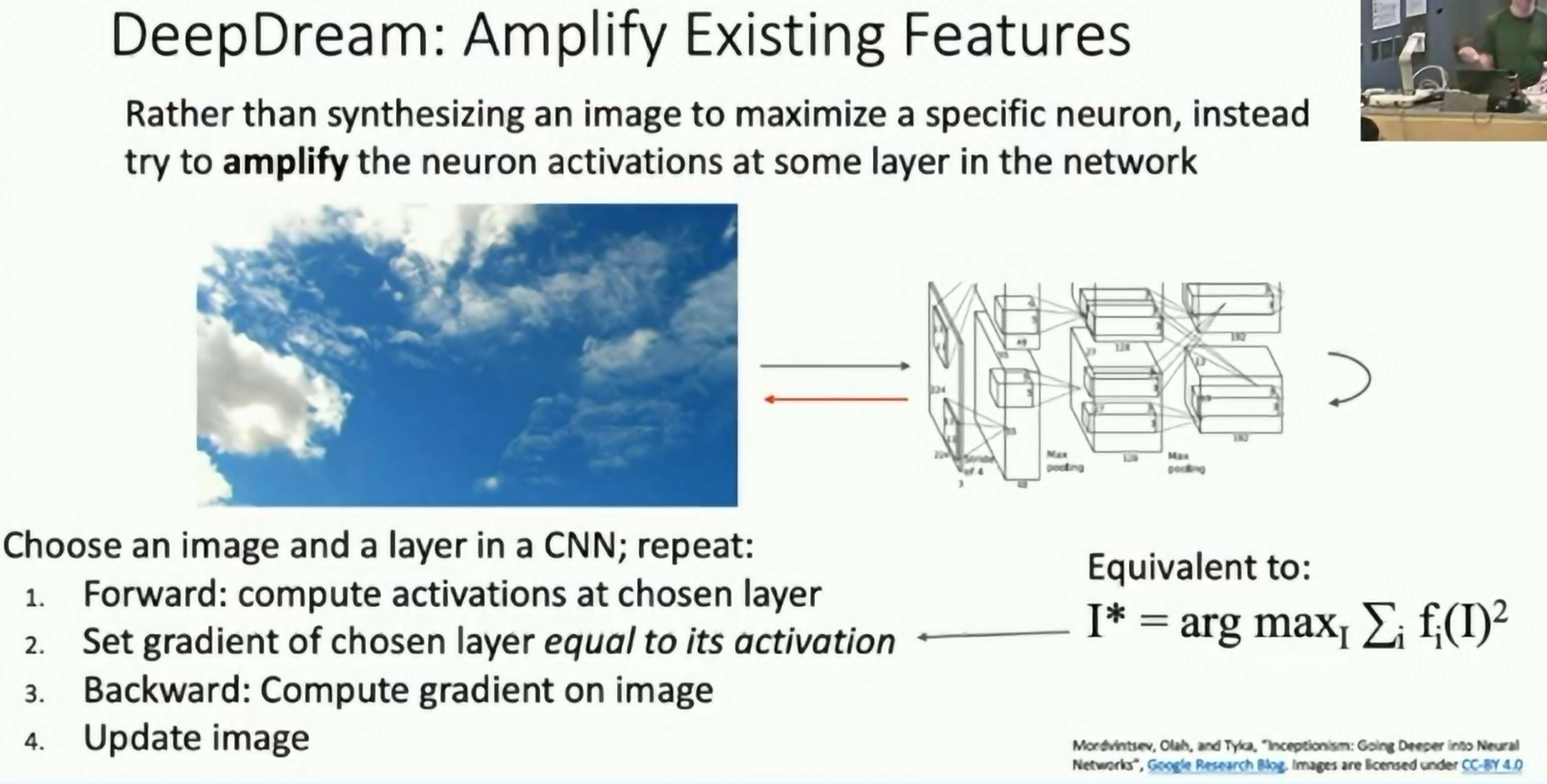
Fig: DeepDream

This needs to get good regularizers to get good results.

DeepDream to lower layer networks:

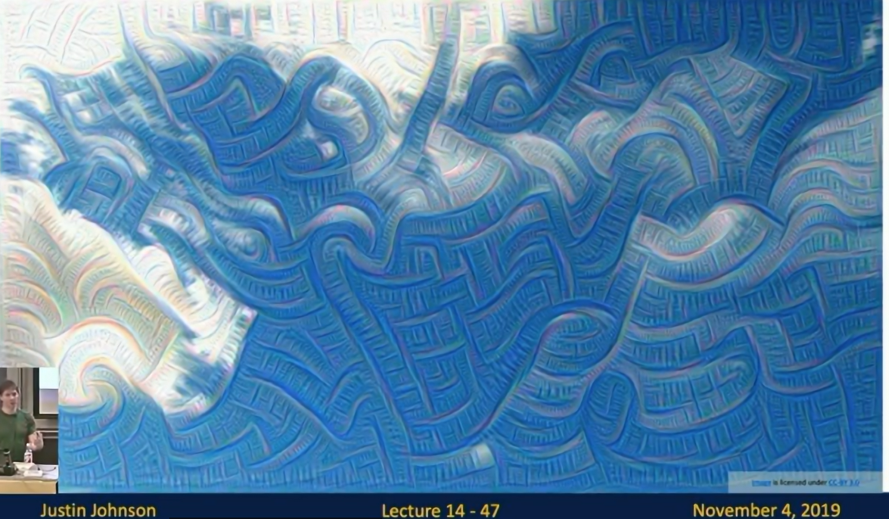
Fig: DeepDream

Higher layers:

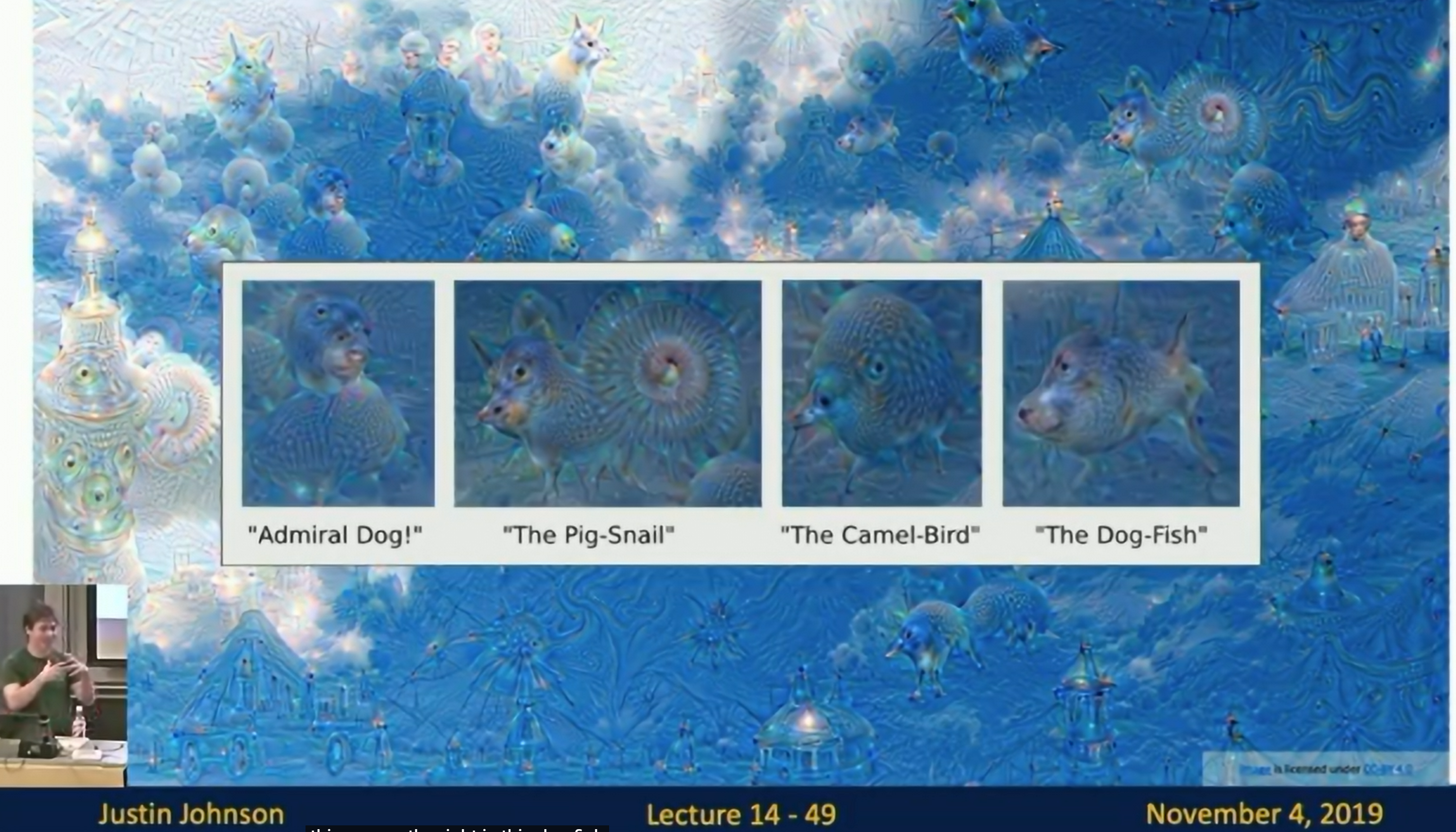
Fig: DeepDream

Patterns are shown out over and over again.

DeepDream for a long time:

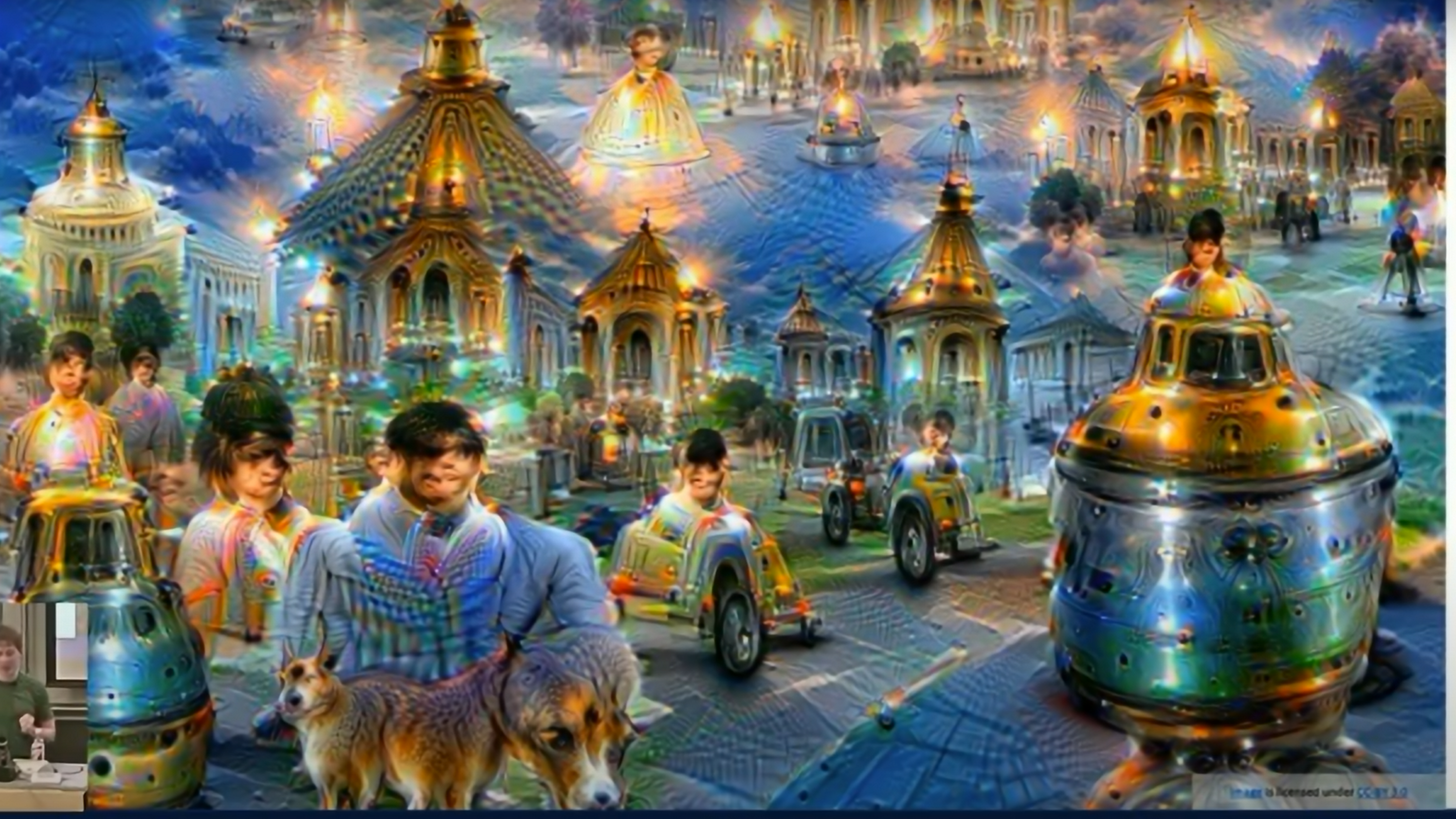
Fig: DeepDream

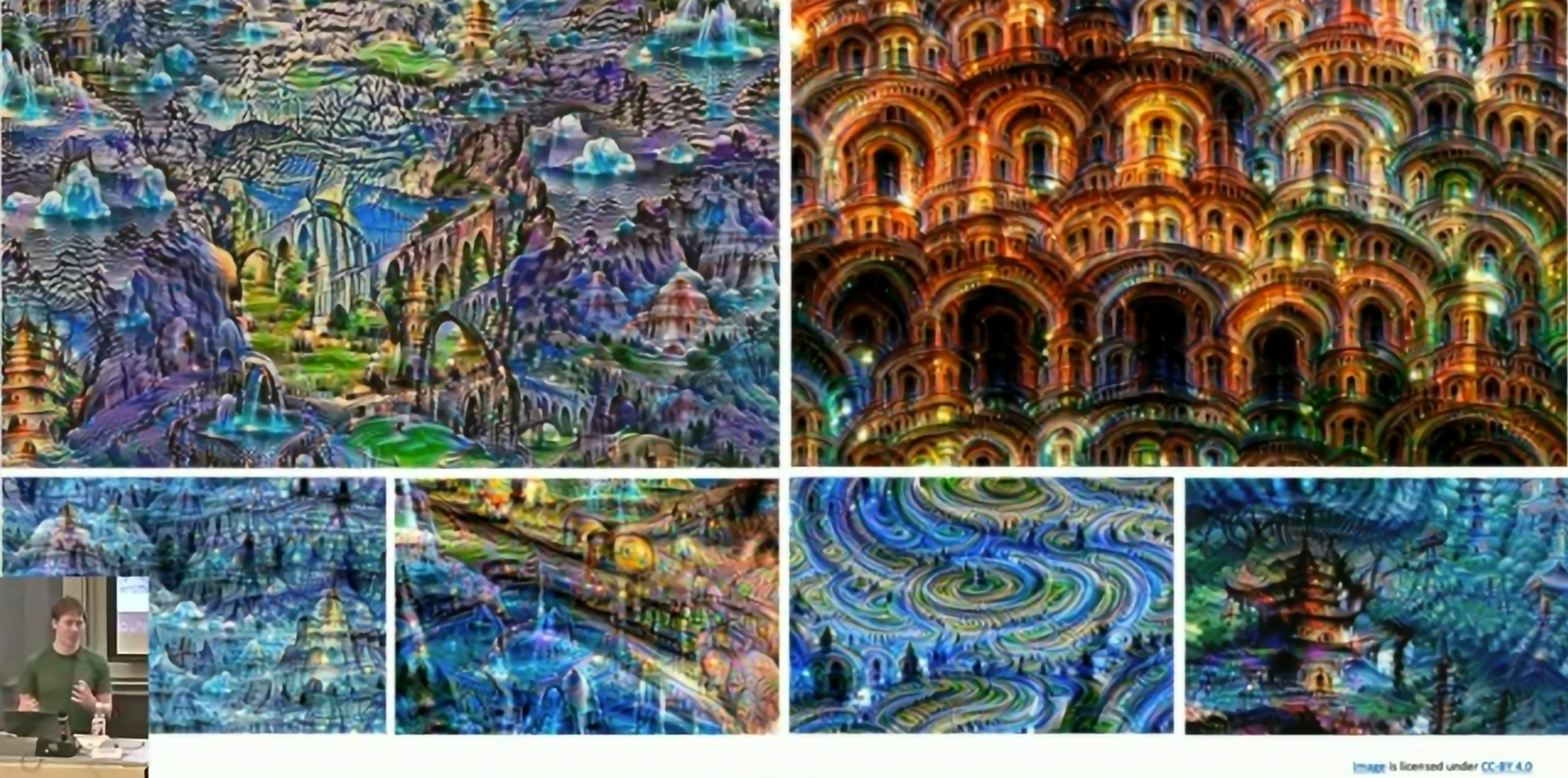
Fig: DeepDream

Application: Texture Synthesis

Nearest Neighbor: SIGGRAPH 2000

Gram Matrix: Correlation. This tells us which features tends to co-occur in the input image. We can perform texture synthesis by matching the Gram matrix using gradient ascent.

Since Gram Matrices are invariant to translation, we can expect to generate textures that are invariant to translation.

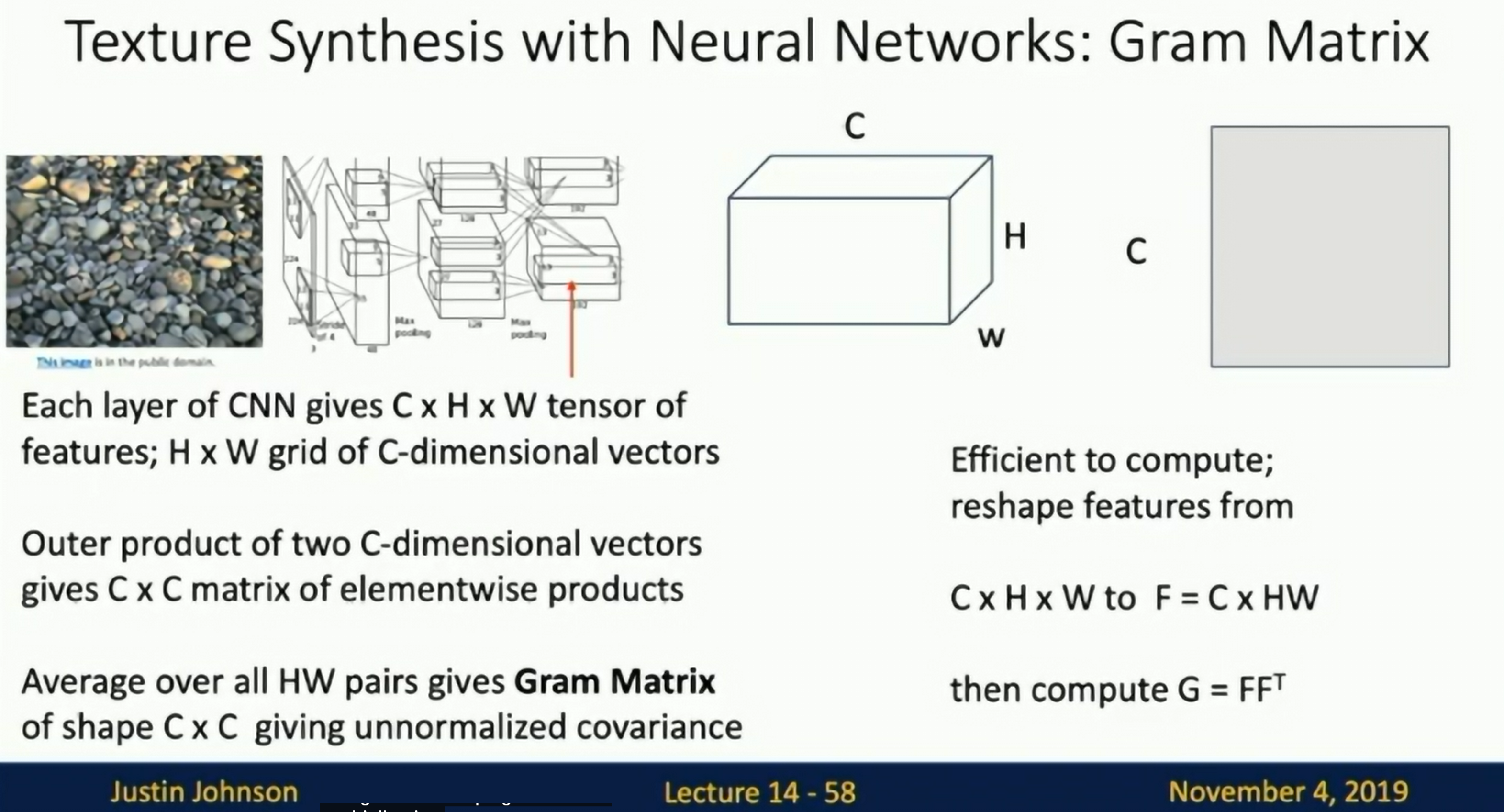
Fig: Texture Synthesis

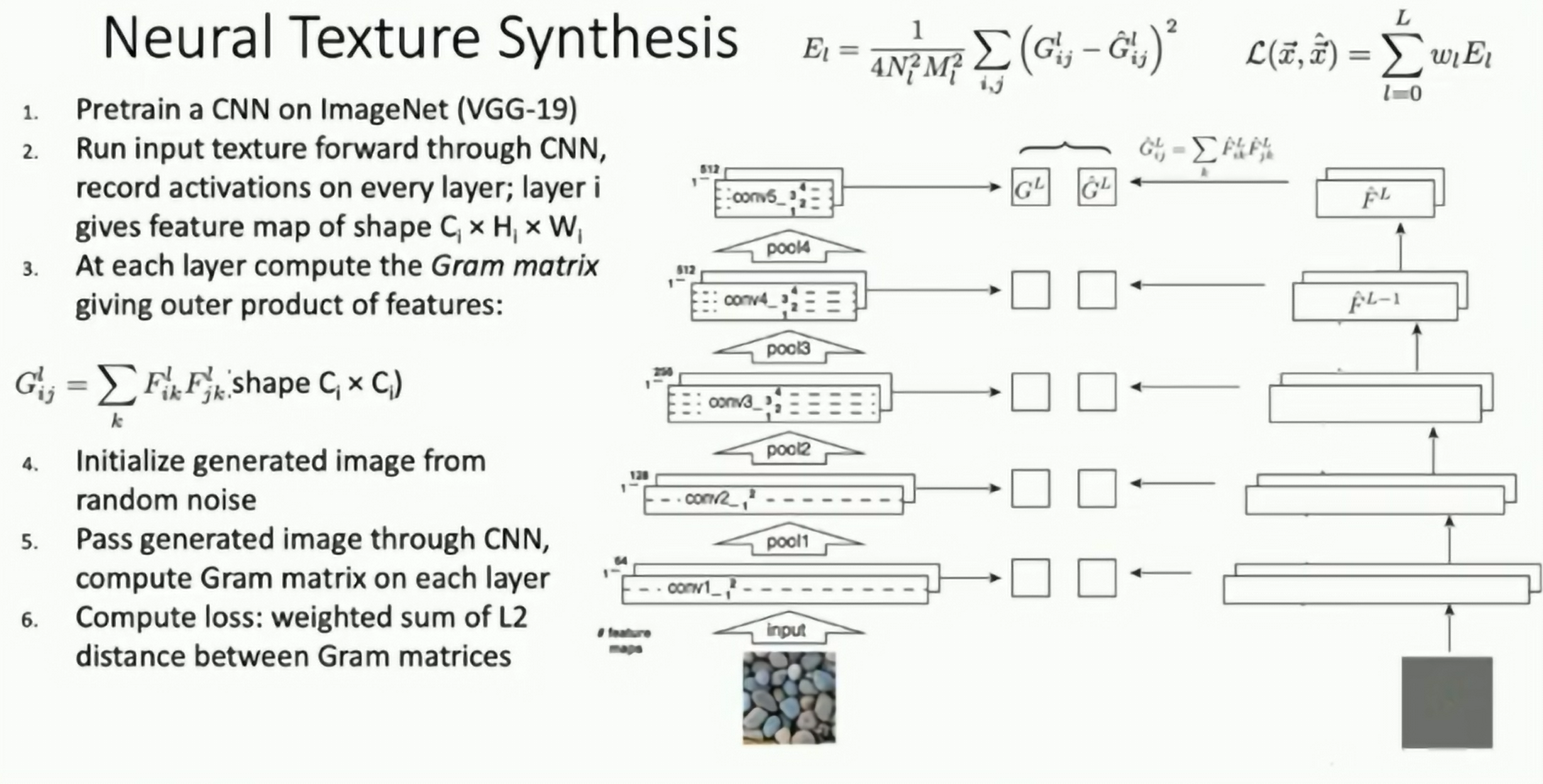
Fig: Texture Synthesis

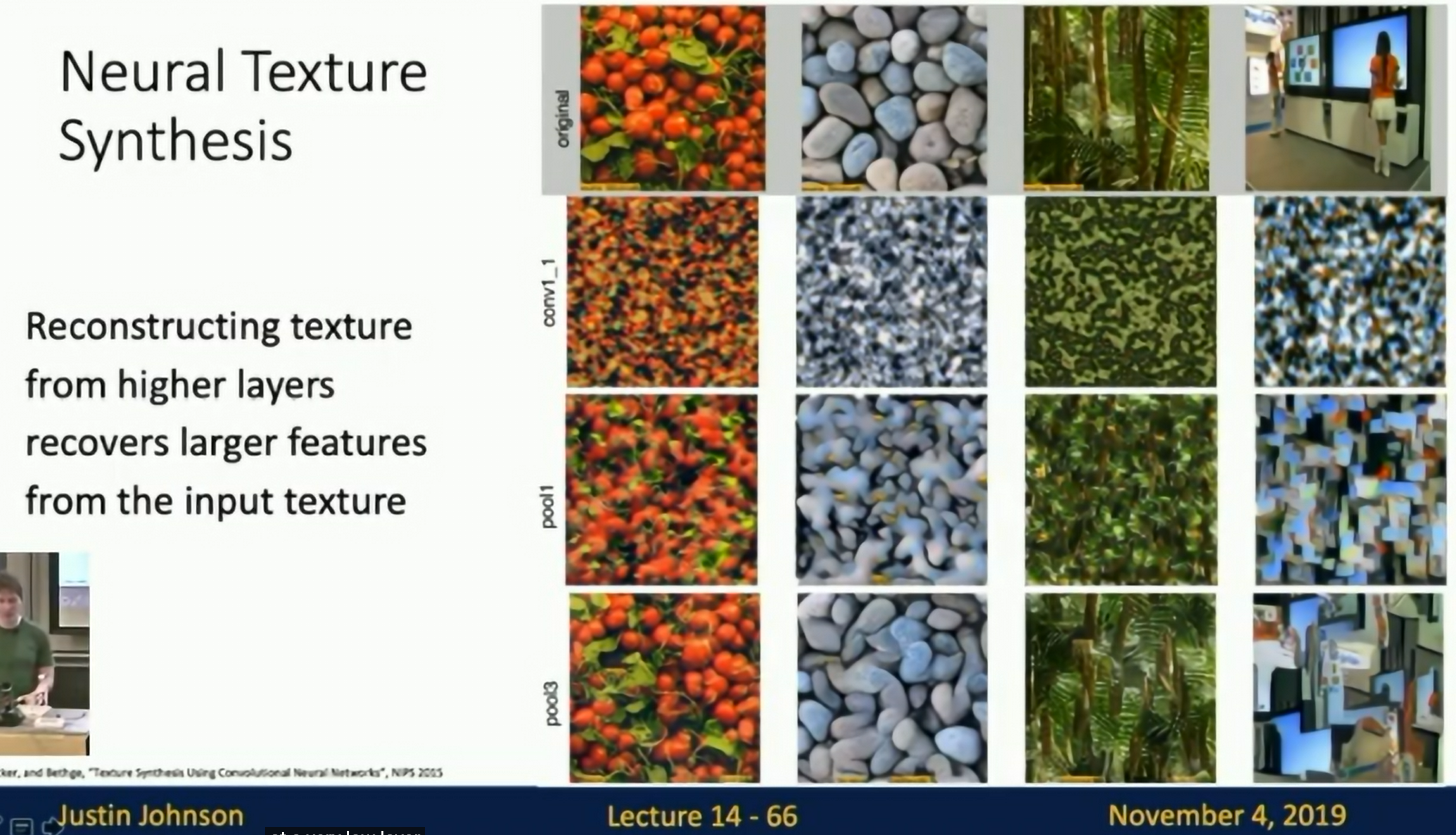
Fig: Texture Synthesis

Application: Style Transfer

Feature + Gram Joint Reconstruction

Content Image + Style Image

CVPR 2016

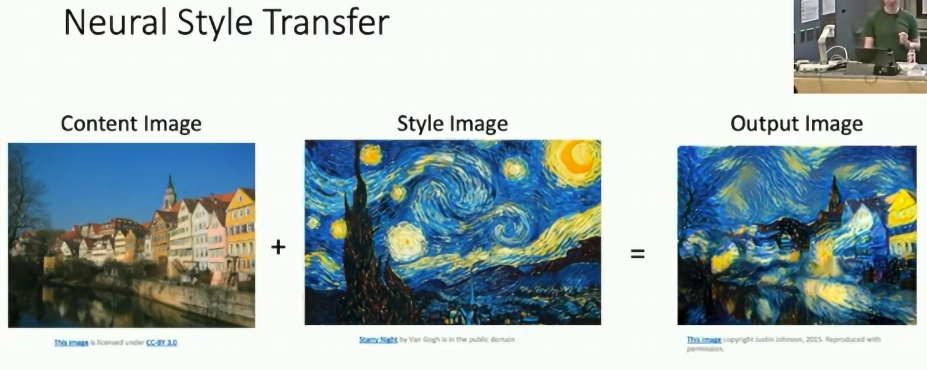
Fig: Style Transfer

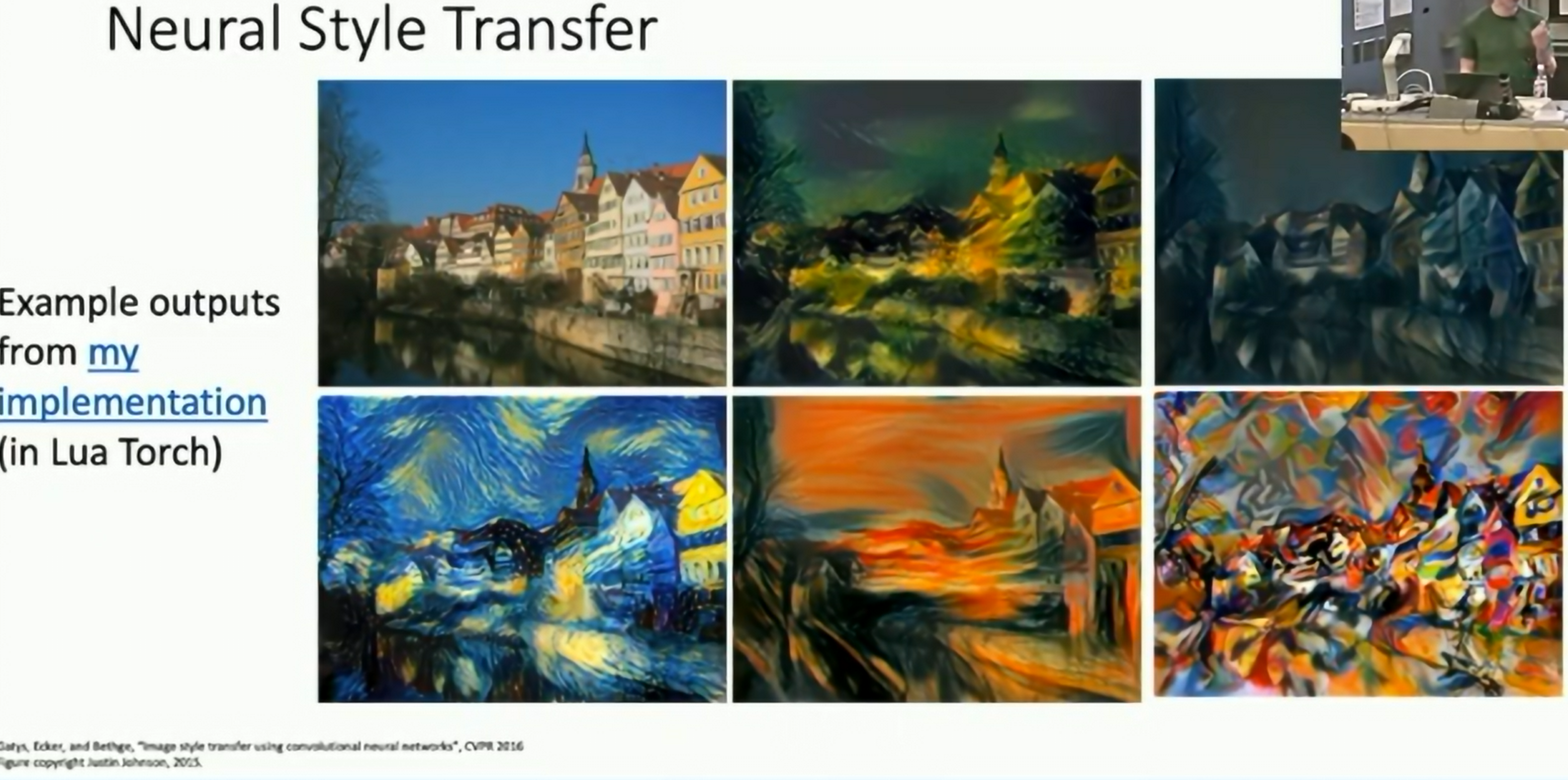
Fig: Style Transfer

We can toggle the weight between the content and style images to get different results.

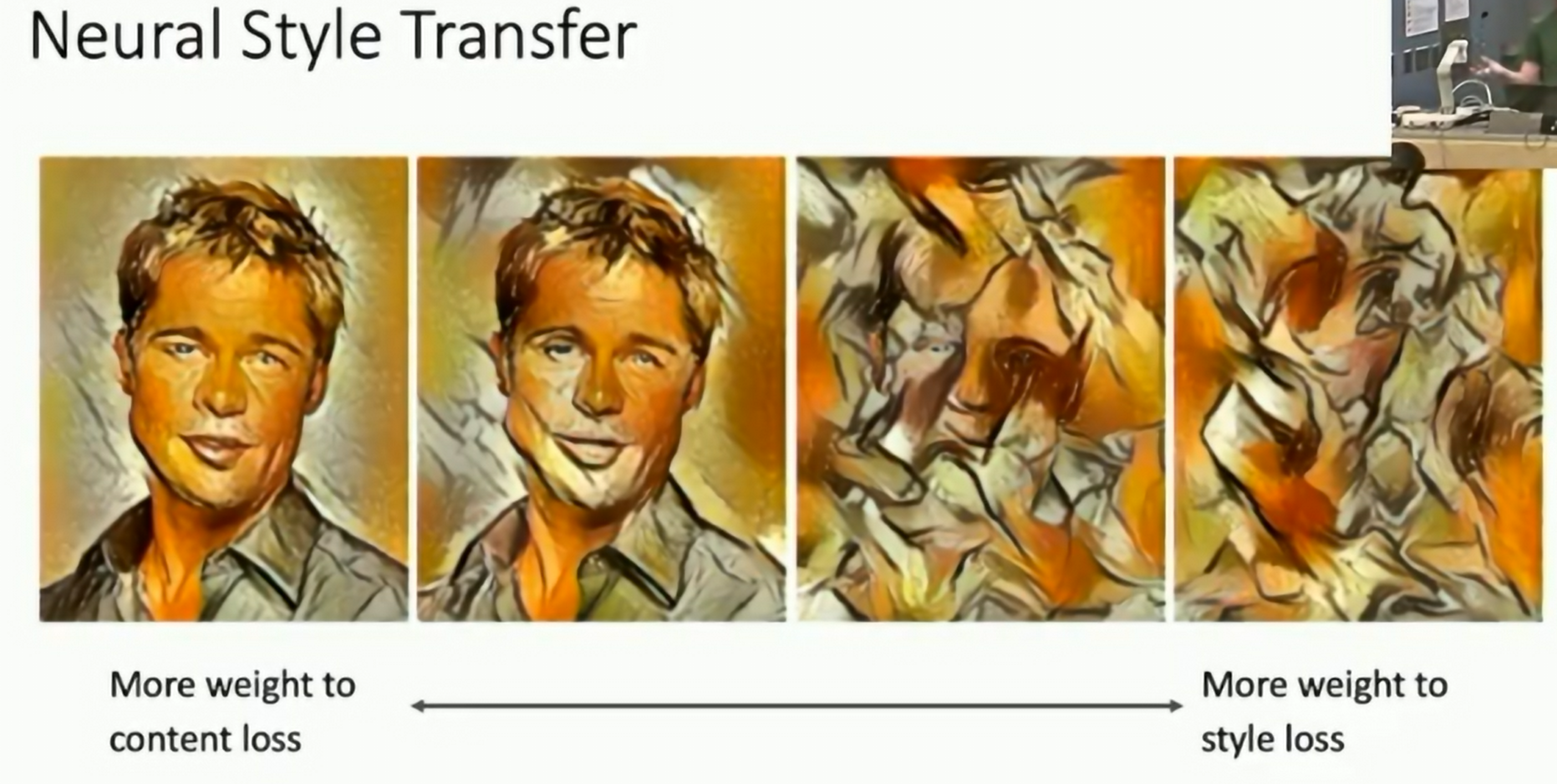
Fig: Style Transfer

Multiple Image Style Transfer:

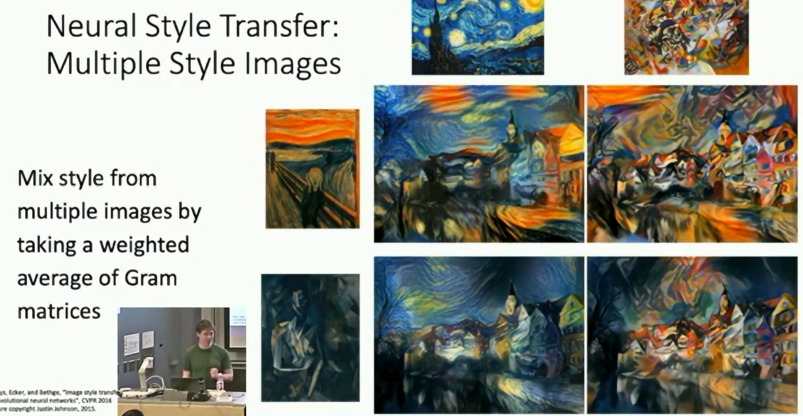
Fig: Style Transfer

Problem: Super slow. Style transfer requires many forward/backward passes through VGG; very slow!

Solution: Train another neural network to perform style transfer.

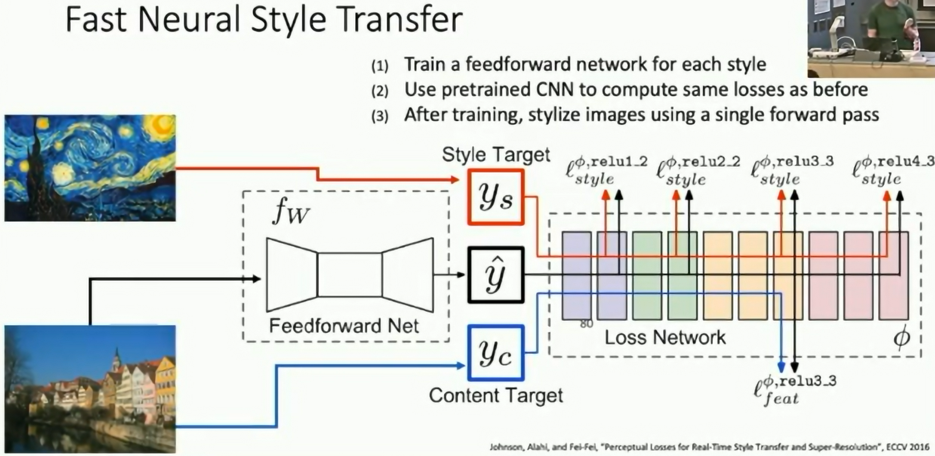
Fig: Style Transfer

Notice on Usage and Attribution

This note is based on the University of Michigan's publicly available course EECS 498.008 / 598.008 and is intended solely for personal learning and academic discussion, with no commercial use.

• Nature of the Notes: These notes include extensive references and citations from course materials to ensure clarity and completeness. However, they are presented as personal interpretations and summaries, not as substitutes for the original course content.
• Original Course Resources: Please refer to the official University of Michigan website for complete and accurate course materials.
• Third-Party Open Access Content: This note may reference Open Access (OA) papers or resources cited within the course materials. These materials are used under their original Open Access licenses (e.g., CC BY, CC BY-SA).
• Proper Attribution: Every referenced OA resource is appropriately cited, including the author, publication title, source link, and license type.
• Copyright Notice: All rights to third-party content remain with their respective authors or publishers.
• Content Removal: If you believe any content infringes on your copyright, please contact me, and I will promptly remove the content in question.

Thanks to the University of Michigan and the contributors to the course for their openness and dedication to accessible education.