Summary: Training neural networks, activation functions, data preprocessing, weight initialization, regularization, learning rate schedules, large batch training, hyperparameter tuning, model ensembles, transfer learning.

@Credits: EECS 498.007 | Video Lecture: UM-CV 5 Neural Networks

Personal work for the assignments of the course: github repo.

Notice on Usage and Attribution

These are personal class notes based on the University of Michigan EECS 498.008 / 598.008 course. They are intended solely for personal learning and academic discussion, with no commercial use.

For detailed information, please refer to the complete notice at the end of this document

One-time setup

Activation functions, data preprocessing, weight initialization, regularization

Activation functions

Activation functions adds critical linearity for neural networks

Sigmoid

$$\sigma(x) = \frac{1}{1 + e^{-x}}$$

• Squashes numbers to range [0,1]
• Historically popular since they have nice interpretation as a starting "firing rate" of a neuron

3 problems:

1. Saturated neurons kill the gradients. (The most problematic aspect)
2. Sigmoid outputs are not zero-centered. Suppose a multi-layer network, then the inputs of all the layers are always positive Also the gradient of this function is always positive. All the gradients for the weights will have the same sign, and gradients will always push the weights into the same direction. This becomes less of a problem when using mini-batches.

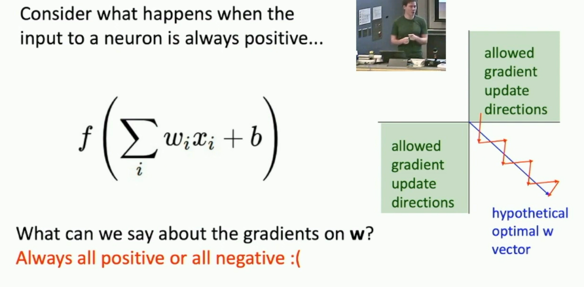
Fig: Gradient update directions

3. exp() is a bit compute expensive: transcendental function. For GPUs, this is not a big deal, the copying takes more time than the computation.

Tanh

$$\tanh(x) = \frac{e^x - e^{-x}}{e^x + e^{-x}} = 2\sigma(2x) - 1$$

• Squashes numbers to range [-1,1]
• zero centered
• still kills gradients when saturated 😦

ReLU

$$\text{ReLU}(x) = \max(0, x)$$

• Does not saturate in the positive region
• Computationally efficient
• Converges much faster than sigmoid/tanh in practice (e.g. 6x)

Problems:

• Not zero-centered output
• Dying ReLU problem: neurons can sometimes be pushed into states in which they become inactive for essentially all inputs. In this case, the gradient flowing through a ReLU neuron is always 0 because the gradient of max(0, x) is 0 if x < 0.

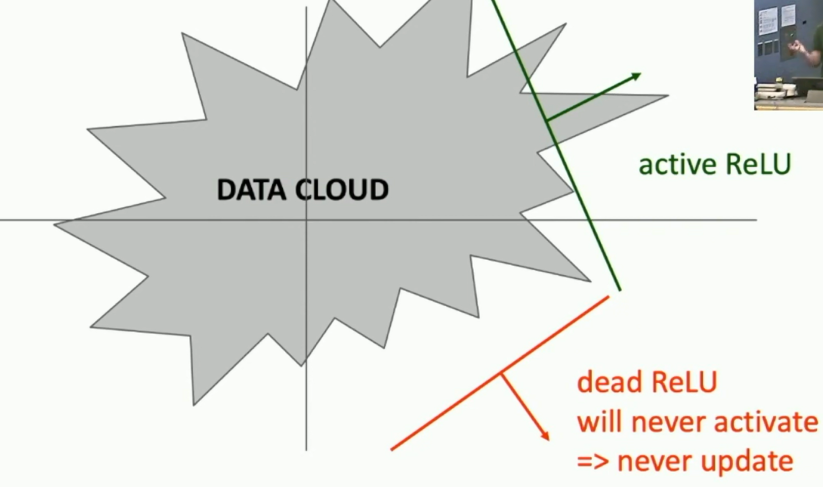
Fig: Dying ReLU problem

dead ReLU will never activate -> never update its weights

Leaky ReLU

Sometimes initialize ReLU neurons with a slightly positive slope in order to mitigate the dying ReLU problem.

$$\text{LeakyReLU}(x) = \max(0.01x, x)$$

• Does not saturate
• Computationally efficient
• Converges much faster than sigmoid/tanh in practice! (e.g. 6x)
• will not "die"

Parametric ReLU (PReLU)

$$\text{PReLU}(x) = \max(\alpha x, x)$$

$\alpha$ is learned and backpropagated through.

Exponential Linear Units (ELU)

$$\text{ELU}(x) = \begin{cases} x & \text{if } x > 0 \\ \alpha(e^x - 1) & \text{if } x \leq 0 \end{cases}$$

• default $\alpha = 1$
• All benefits of ReLU
• Closer to zero mean outputs
• Negative saturation regime compared with ReLU

Problem:

• Computationally more expensive

SELU

A rescaled version of ELU

$$\text{SELU}(x) = \lambda \begin{cases} x & \text{if } x > 0 \\ \alpha(e^x - 1) & \text{if } x \leq 0 \end{cases}$$

where $\alpha = 1.6732632423543772848170429916717$

and $\lambda = 1.0507009873554804934193349852946$

• Scaled version of ELU that works better for deep networks
• Self-normalizing property: SELU activations preserve mean and variance of inputs. Can train deep SELU neural networks without normalization layers.

Comparison of activation functions

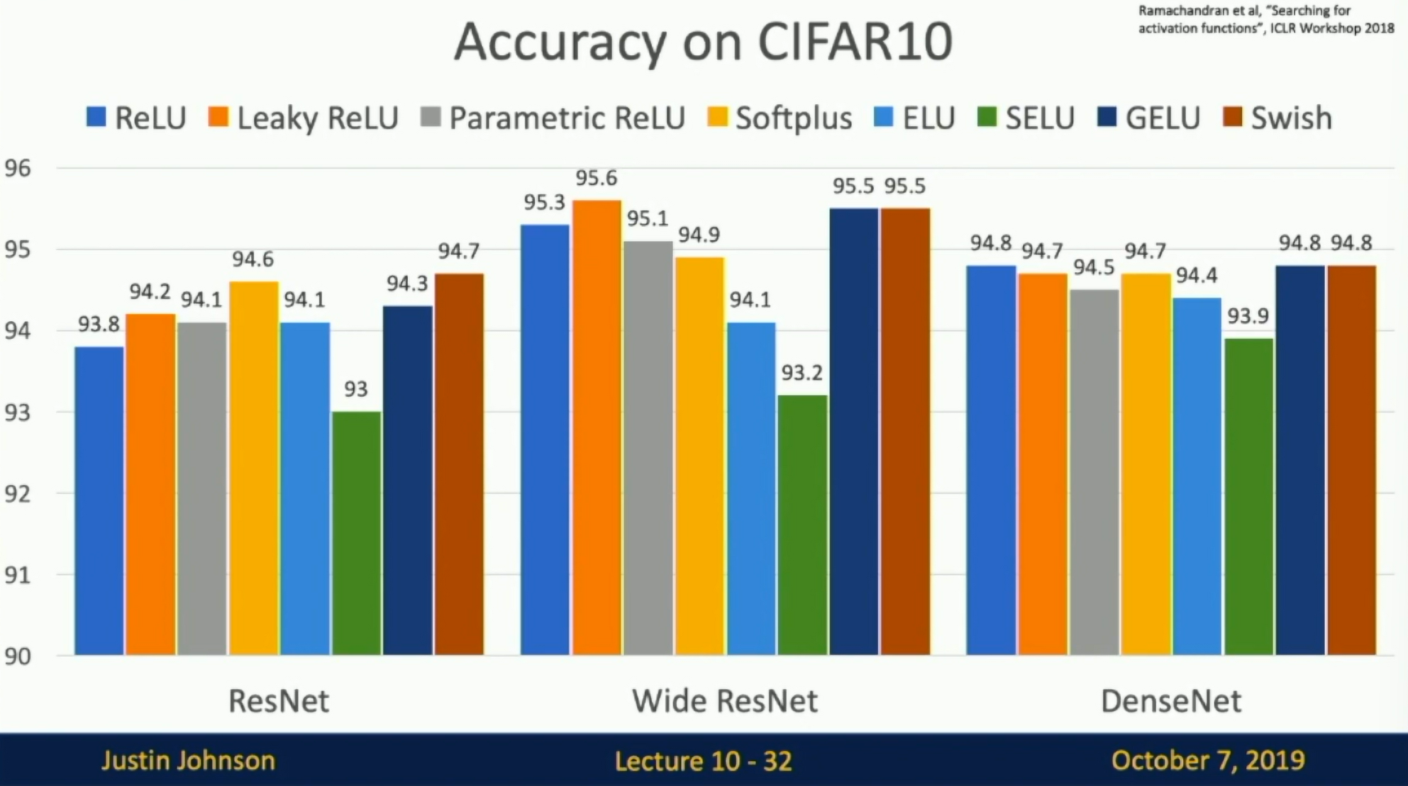
Fig: Comparison of activation functions

Summary:

• Don't think too hard. Just use ReLU.
• Try out Leaky ReLU/ELU/SELU/GELU if you need to squeeze that last 0.1%
• Don't use sigmoid or tanh. The models will learn very slowly.

Data preprocessing

We want to normalize the inputs to have zero mean and unit variance. This helps the model learn faster and prevents the gradients from going out of control.

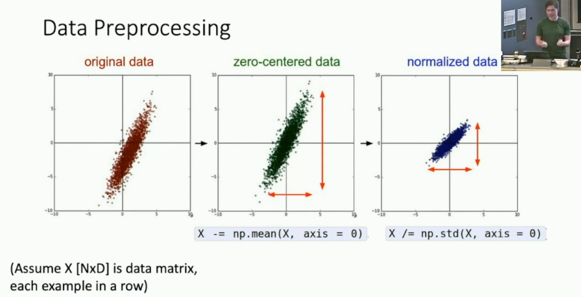
Fig: Data preprocessing

In practice, you may also see PCA and Whitening applied to the data.

Rotate the data so that the principal components are aligned with the axes. This is called PCA whitening. For image data this is not so common.

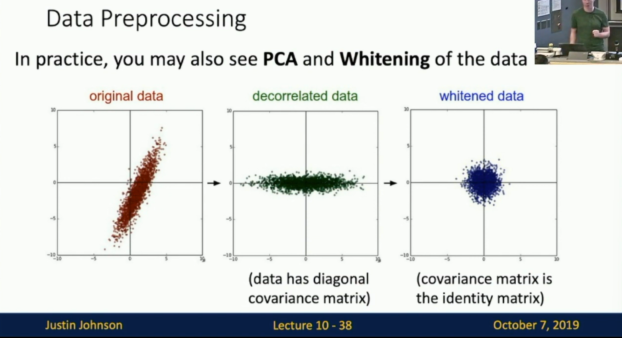
Fig: PCA whitening

Why do we need to normalize the data?

Classification loss would be very sensitive to changes in weight matrix; hard to optimize.

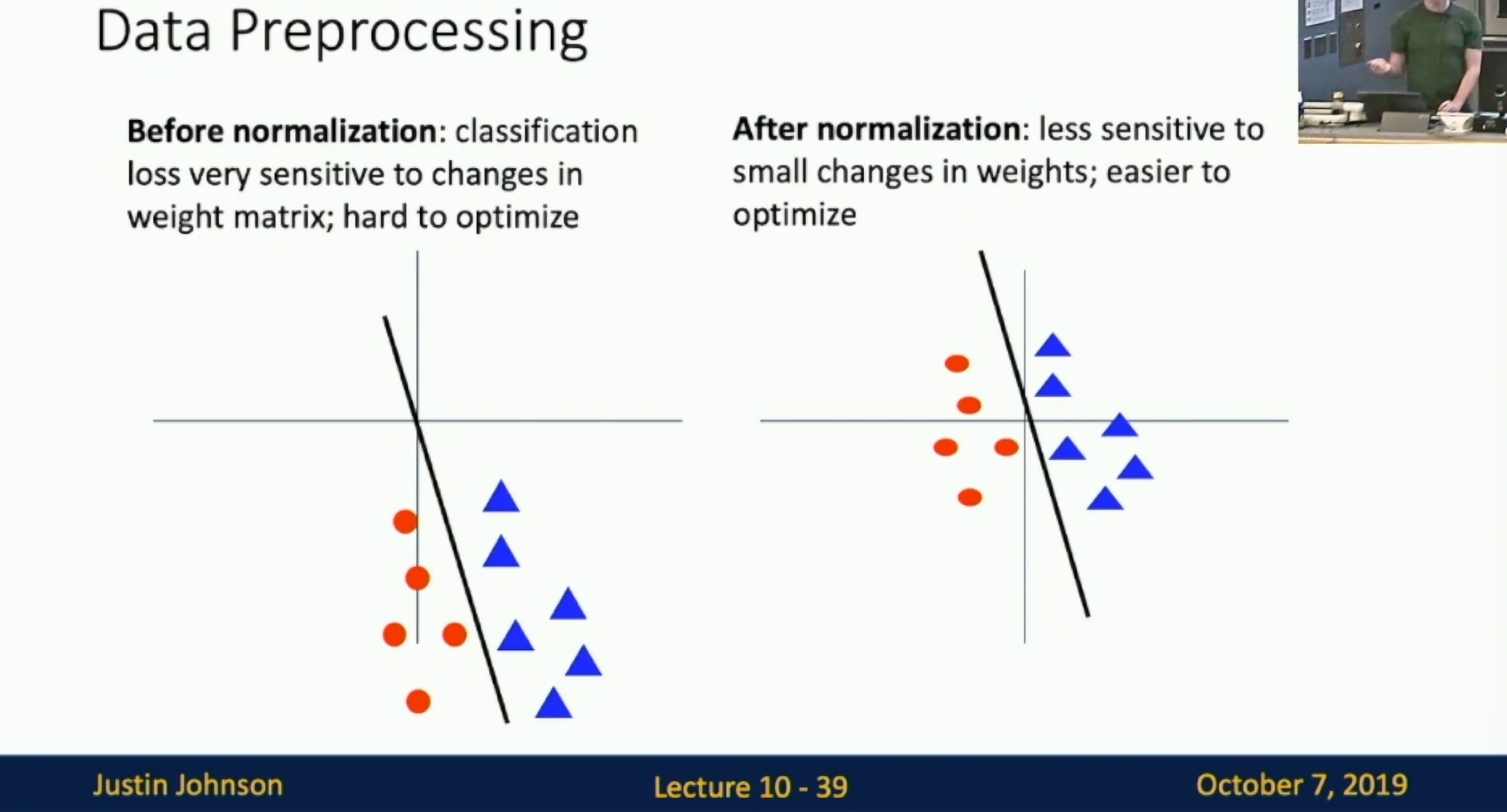
Fig: Classification

Real examples

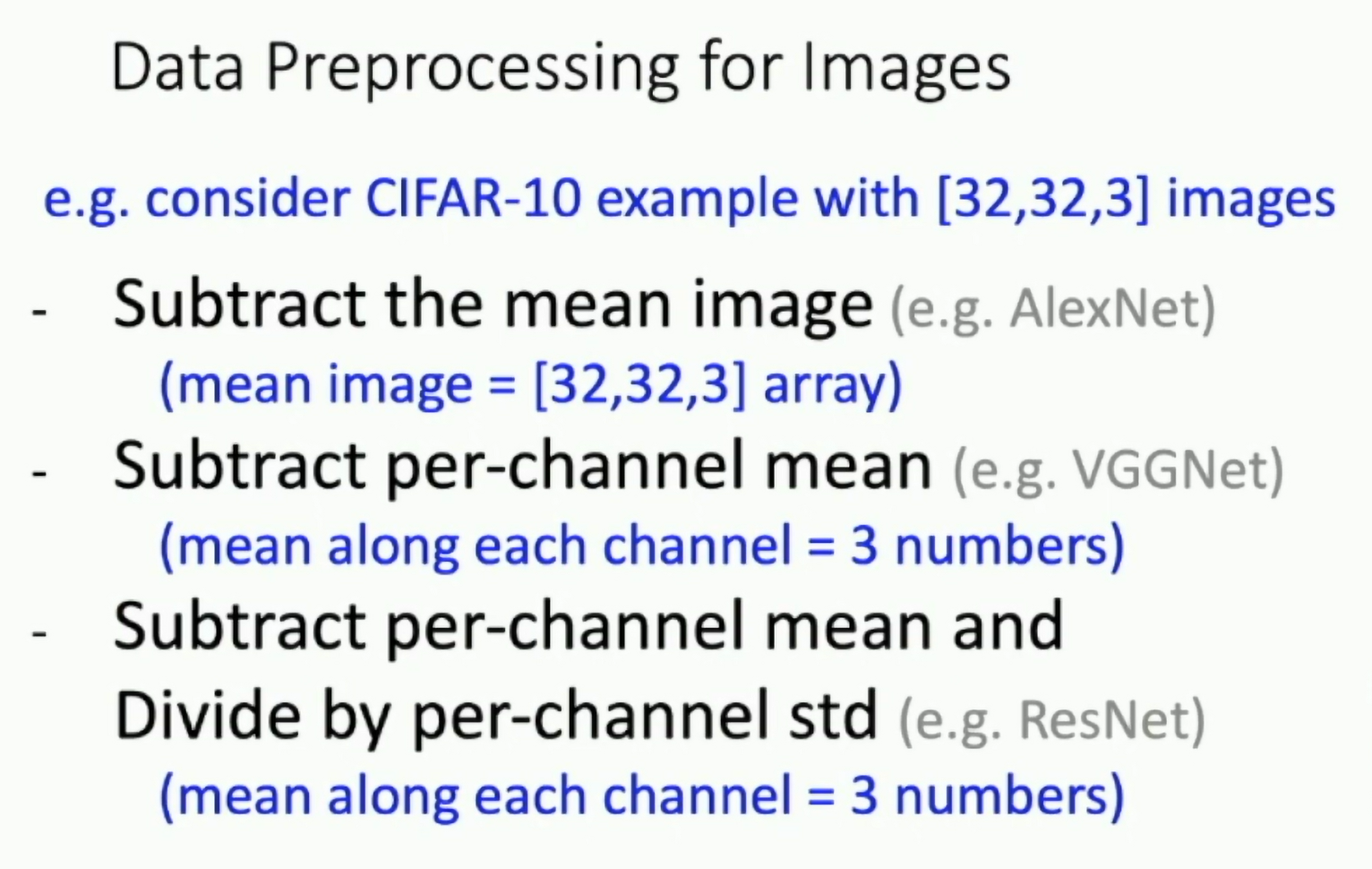
Fig: Real examples

Weight initialization

Zero initialization is bad because all neurons will have the same gradient and will update in the same way.

Weight Initialization: small random numbers. Fairly ok with shallow networks, but problems with deeper networks.

This is to ensure that the gradient behaves nicely at the beginning of training.

Activation Statistics: Histogram of each layers

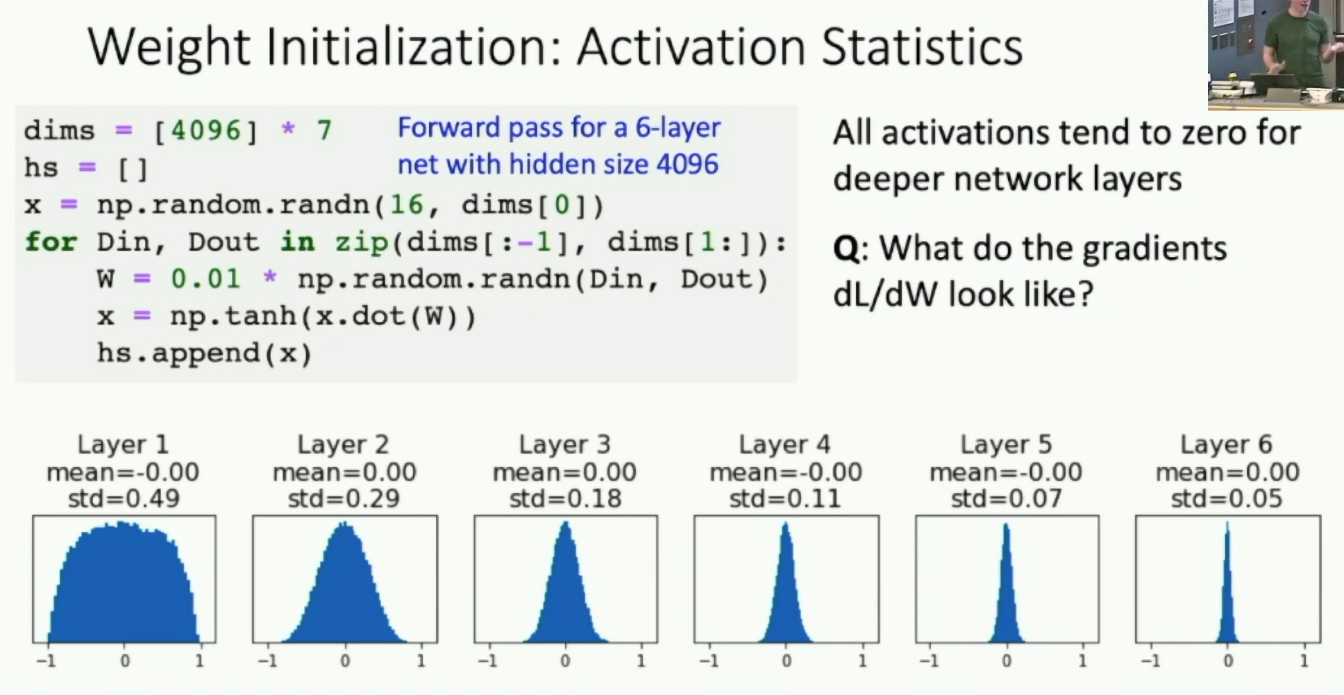
Fig: Statistics of a sample x

Problem: This initialization may be too small for deep networks.

If we initialize the weights too big, all neurons will be saturated and the gradients will be zero.

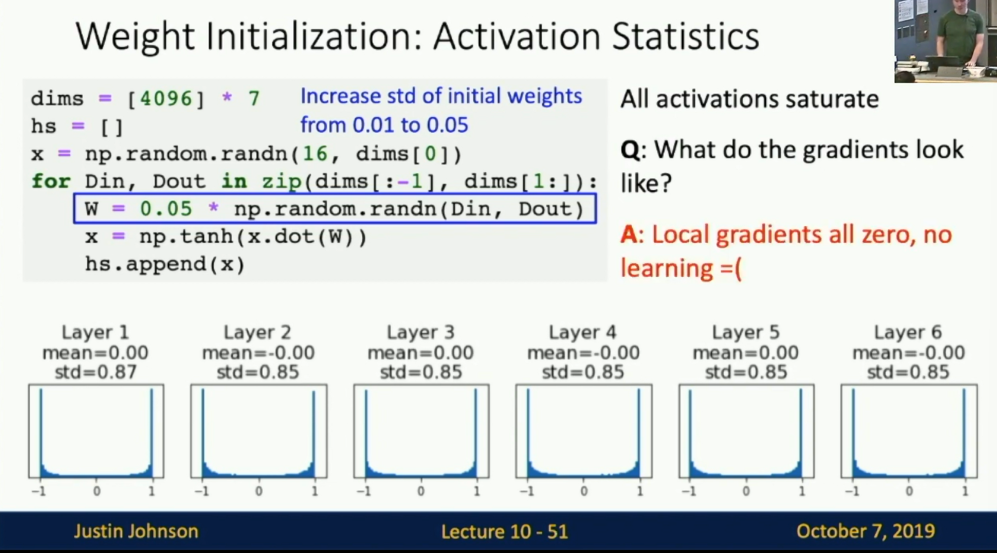
Fig: Statistics of a sample x when weights are too big

Xavier initialization

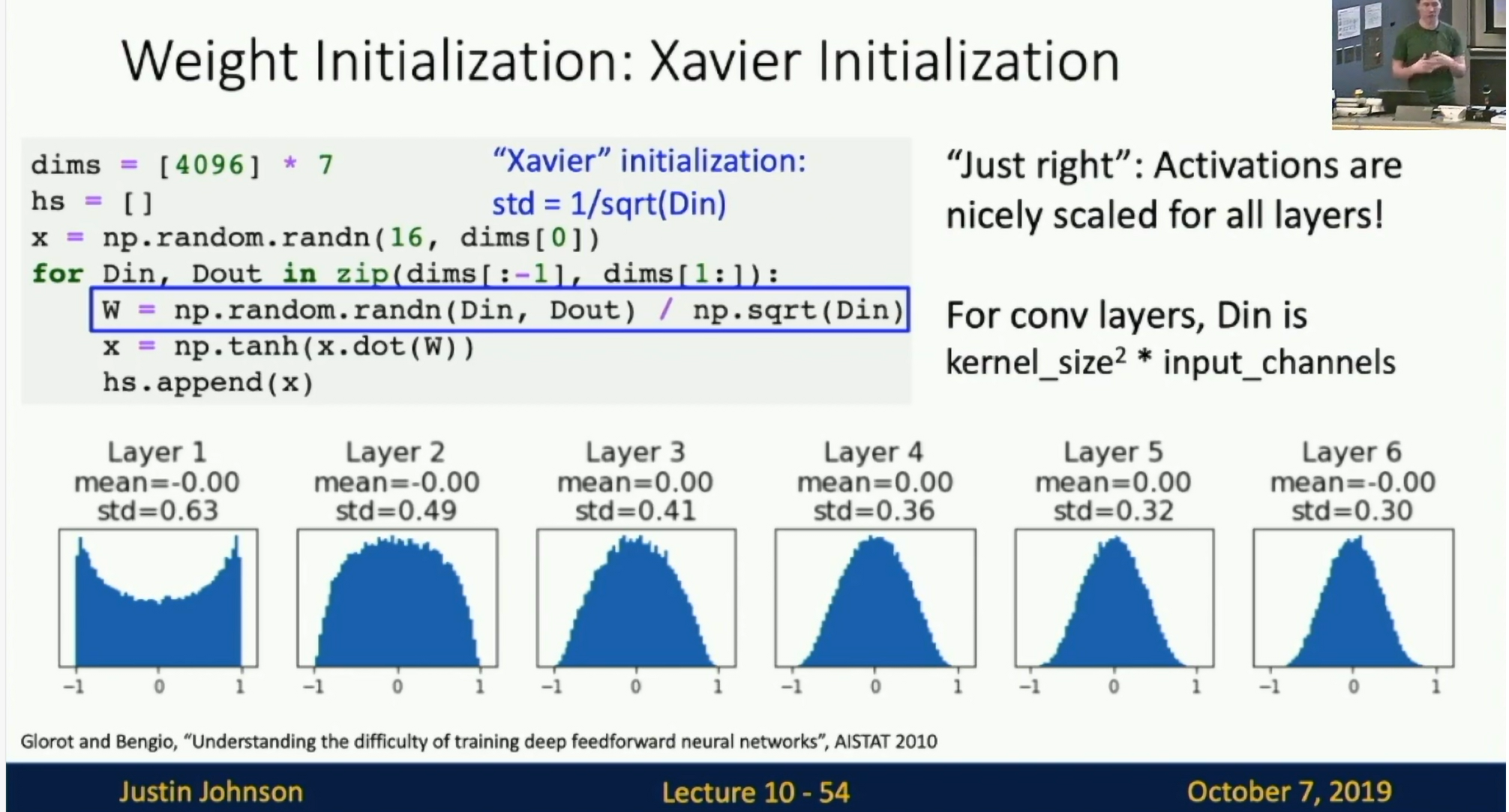
Fig: Xavier initialization

Derivation: Variance of output = Variance of inputs

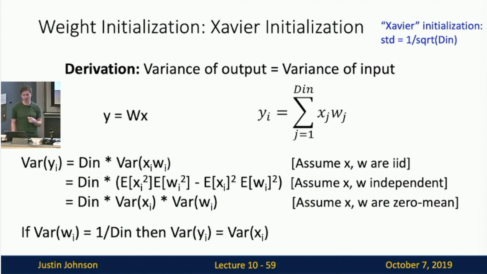
Fig: Derivation

We are only taking about linear layers. For ReLU, this method will collapse to zero again, no learning 😦

Kaiming/MSRA initialization

Multiply Xavier by $\sqrt{2}$ for ReLU activation functions.

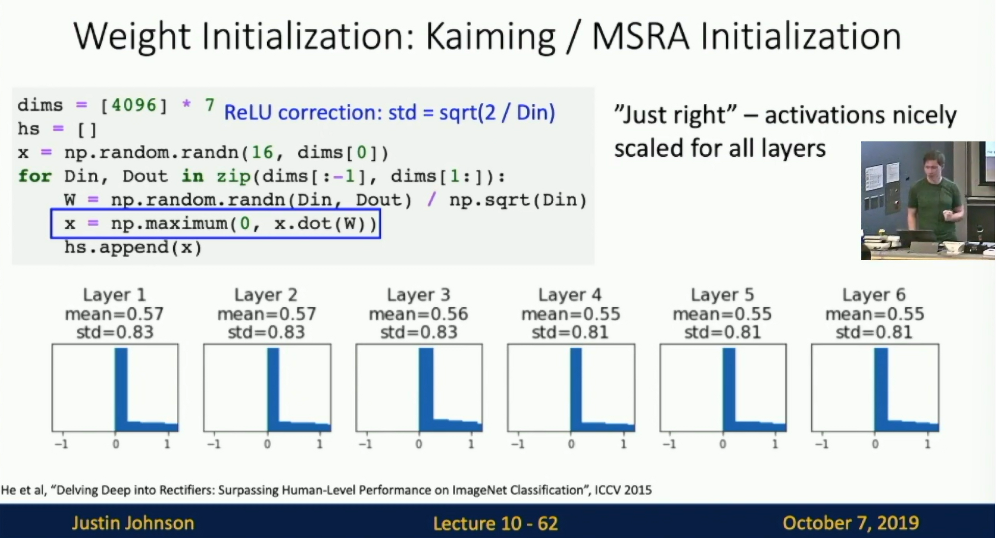
Fig: Kaiming/MSRA initialization

This keeps the variance of the output the same as the variance of the input.

This is sufficient to got VGG to train from scratch.

Residual Networks

MSRA is not that useful for residual networks.

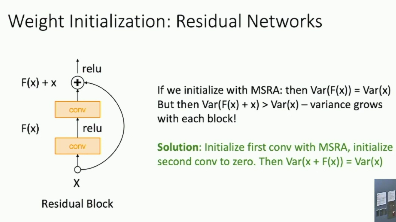
Fig: Residual Networks

Regularization

Add term to the loss.

Weight decay

$$L = \text{data loss} + \lambda R(W)$$

In common we use:

• L2 regularization: $R(W) = \sum_i W_i^2$ (weight decay)
• L1 regularization: $R(W) = \sum_i |W_i|$
• Elastic net: $R(W) = \alpha \sum_i |W_i| + \beta \sum_i W_i^2$ (L1 + L2)

Dropout

Randomly set some neurons to zero during forward and backward pass.

We want to prevent the network from relying too much on any one neuron. Prevents co-adaptation of neurons.

Another interpretation: Ensemble of networks. Dropout is like training an ensemble of networks and averaging their predictions.

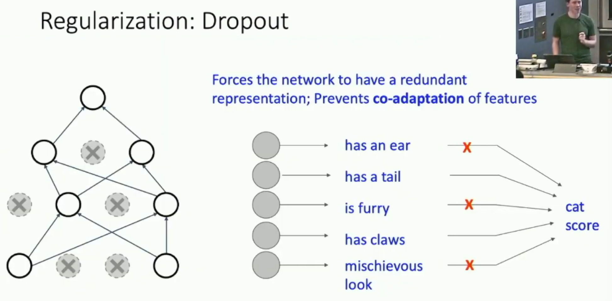
Fig: Dropout

Problem: Test time. We want to use all the neurons.

We average out the randomness at test-time, but this integral seems hard... So we need to approximate the integral.

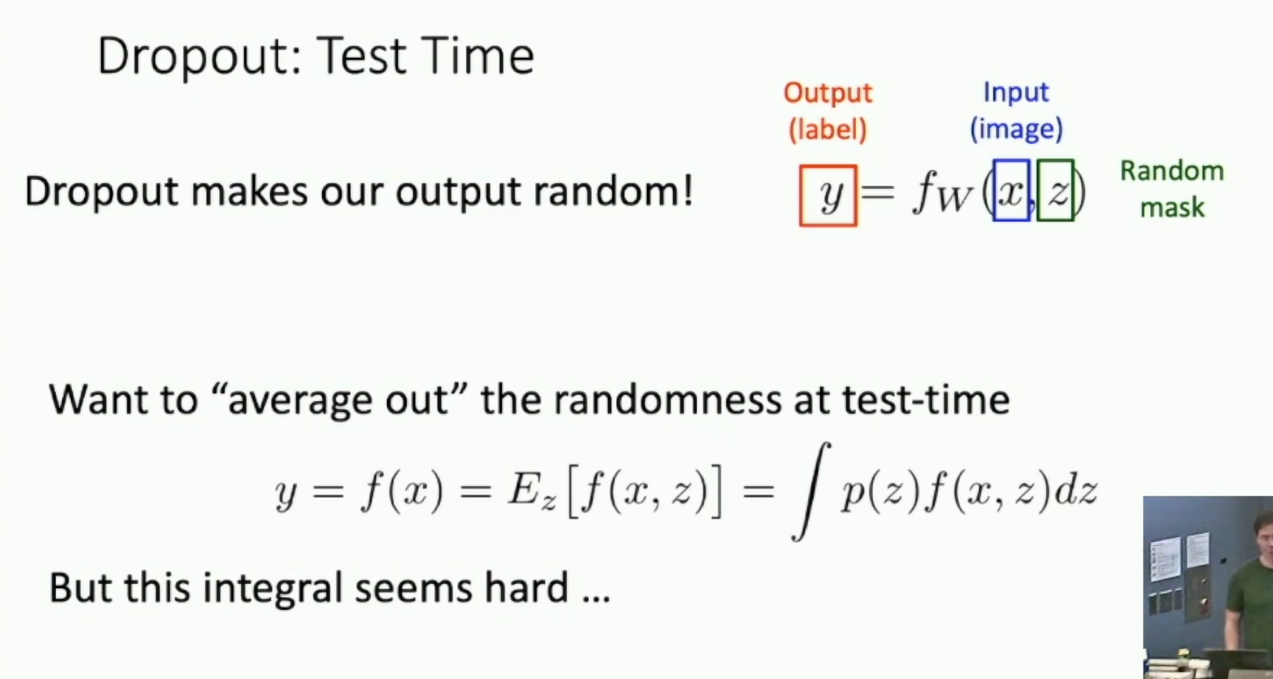
Fig: Dropout at test time

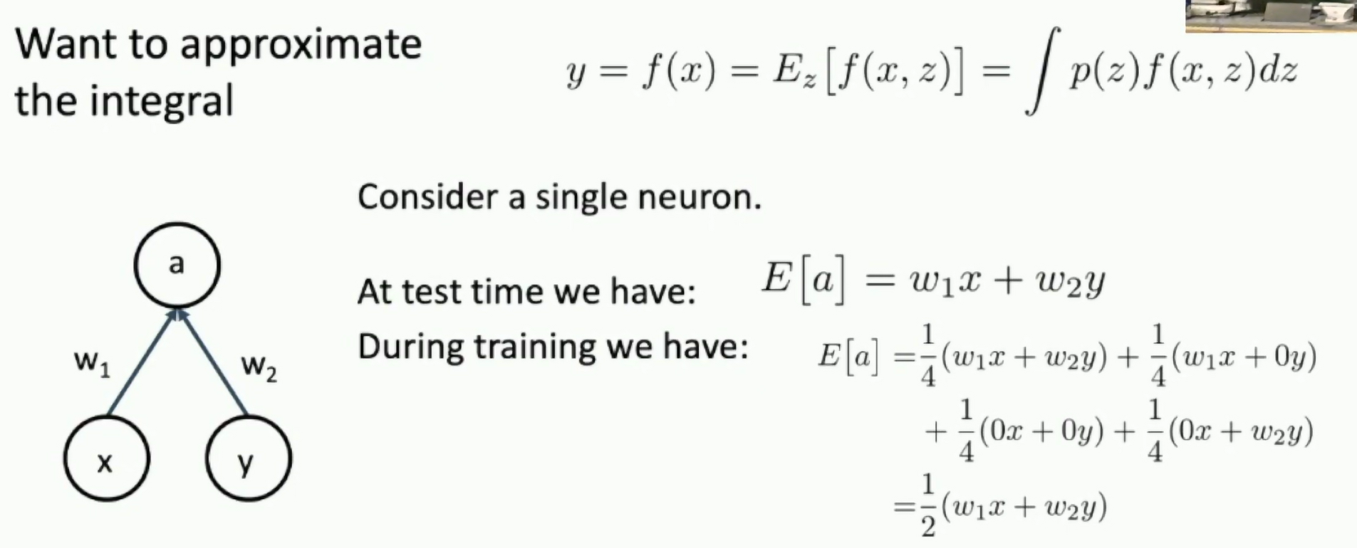
Fig: Dropout at test time

At test time, we multiply the weights by the dropout probability.

At test time all neurons are active always. => We must scale the activations so that for each neuron, the expected output is the same as the expected output at training time.

Drop in forward pass, scale in backward pass.

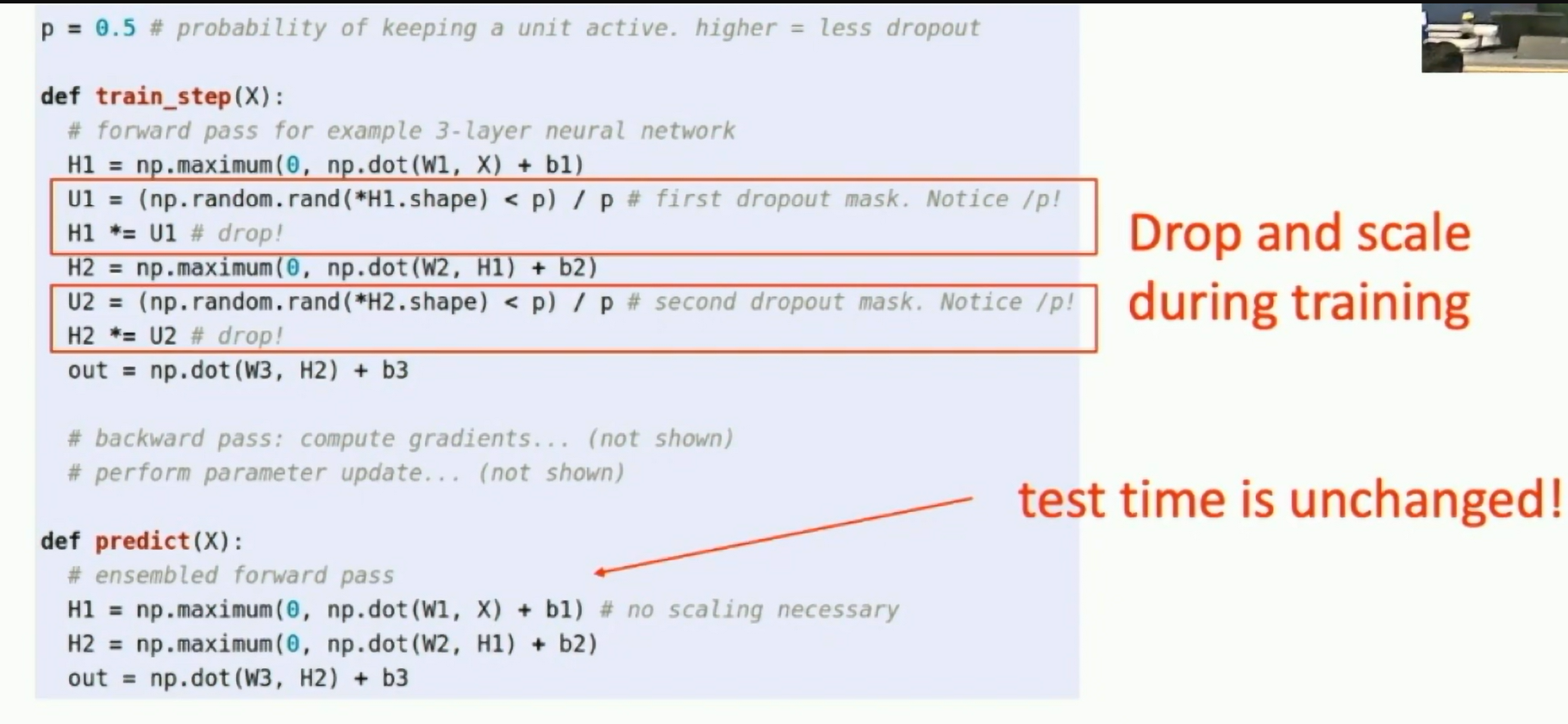
Fig: Inverted dropout

Dropout architecture is not common in modern architectures.

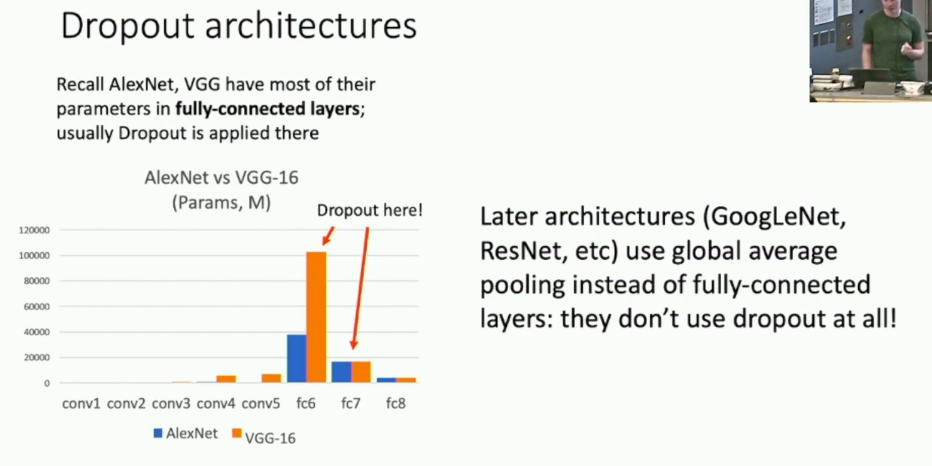
Fig: Dropout at test time

Batch normalization

We have already learned this in the previous lecture.

For ResNet and later, often L2 and batch normalization are the only regularizers!

Data Augmentation

• Random crops
• Random flips
• Random scales
• Color jittering

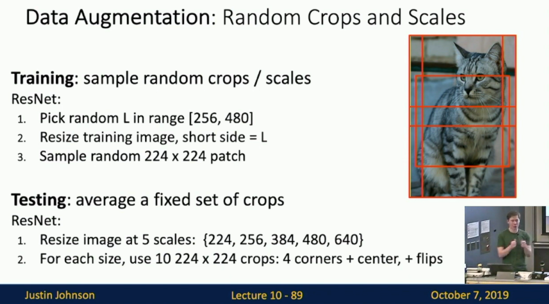
Fig: Data Augmentation

Get creative for you problem!

Random mix/combinations of:

• Translation
• Rotation
• Stretching
• Shearing
• lens distortions,... (go crazy)

Other regularizers

DropConnect

Training: Instead of dropping out neurons, drop out weights. Testing: Use all the connections.

Fractional Max Pooling

Training: Randomize the size of the pooling region. Testing: Average predictions over different samples.

Stochastic Depth

Training: Skip some residual blocks in ResNet.

Testing: Use the whole network.

Stochastic Depth

Training: Set random images regions to 0 Testing: Use the whole image

Mixup

Training: Train on random blends of images Testing: Use original images

Training dynamics

learning rate schedules, large batch training, hyperparameter tuning

Learning rate schedules

Starting with hight learning rate and lower it over time.

Common schedules:

• Step decay: lower the learning rate by a factor every few fixed epochs.

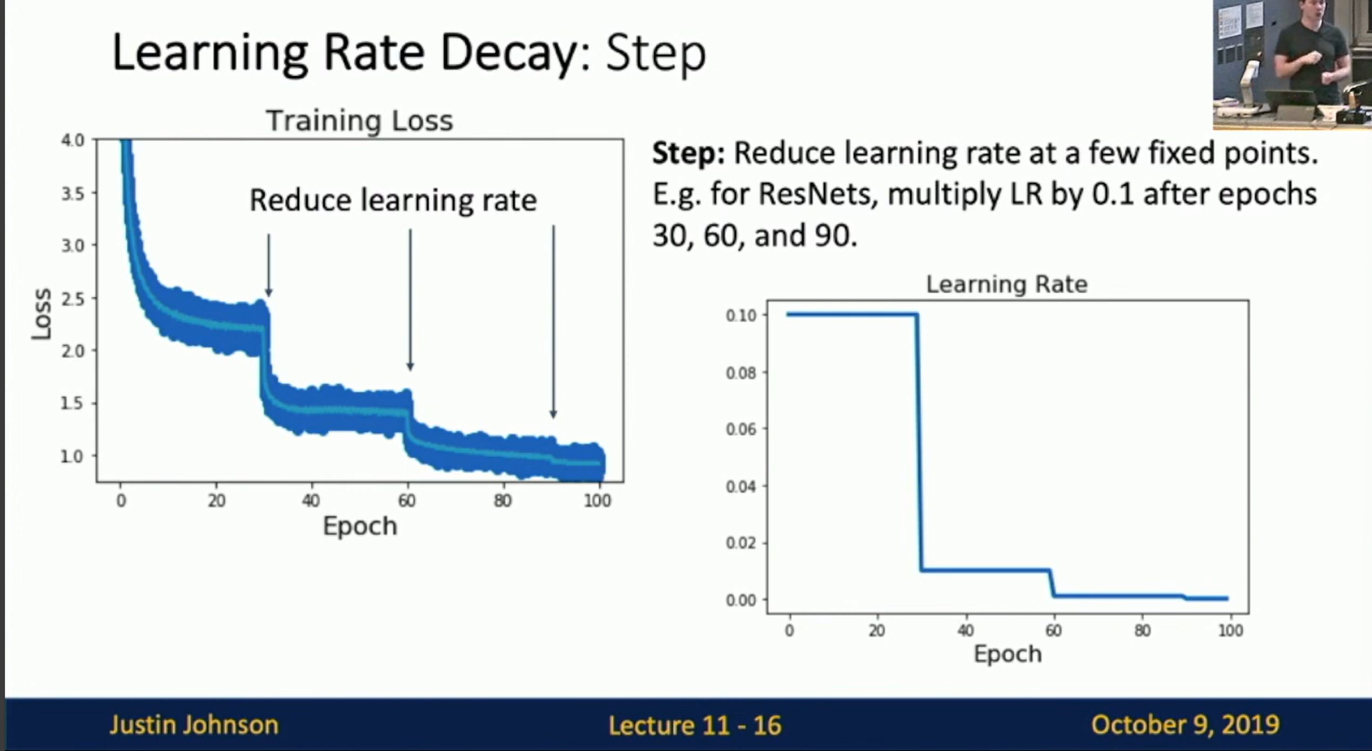
Fig: Step decay

- Cosine: lower the learning rate according to a cosine schedule. This has less hyperparameters than step decay. Often used for CV.

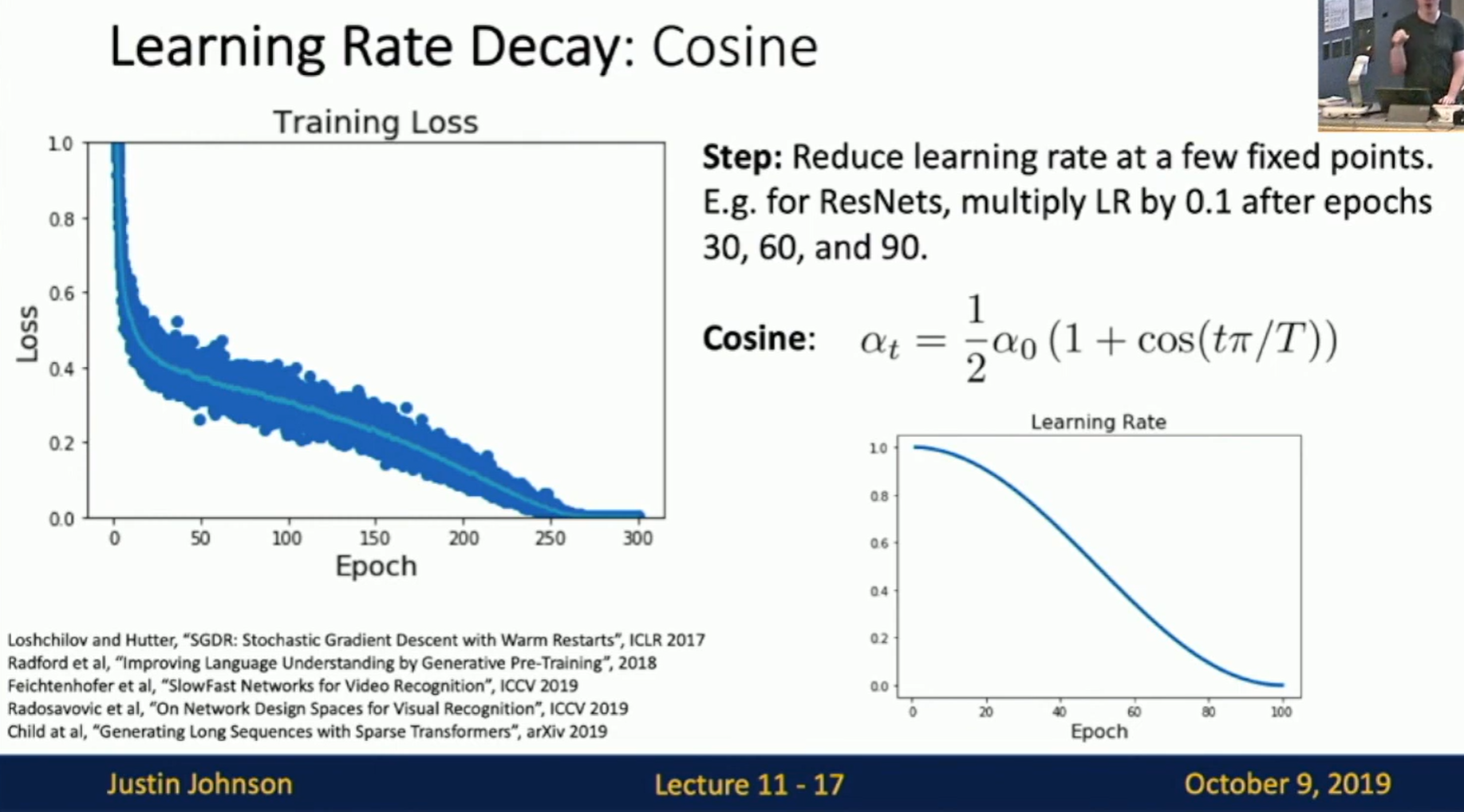
Fig: Cosine

• Linear: linearly decrease the learning rate over time. Often used for NLP.
• Inverse square root: $\frac{\alpha}{\sqrt{t}}$ where $\alpha$ is the initial learning rate and $t$ is the iteration number.
• Constant: keep the learning rate constant. This works already quite well. A constant schedule is often used for fine-tuning. Adam is already adaptive.

Tip: torch.zero_grad() is important. If you don't zero the gradients, the gradients will accumulate.

Usually for Classification problem, the loss will not explode after a long time, but this is possible for other problems, e.g. Reinforcement Learning. (General experience)

Early stopping

Stop training the model when accuracy on the validation set decreases, or train for a long time, but always keep track of the model snapshot that worked best on val. Always a good idea to do this!

Choosing hyperparameters

Grid search

Choose several values for each hyperparameter often chosen log-linearly. Evaluate all possible choices on this hyperparameter grid.

Random search

Choose several intervals for each hyperparameter often chosen log-linearly.

Run many different trails randomly.

This allow us to sample more hyperparameters along one dimension. This is useful when one hyperparameter is more important.

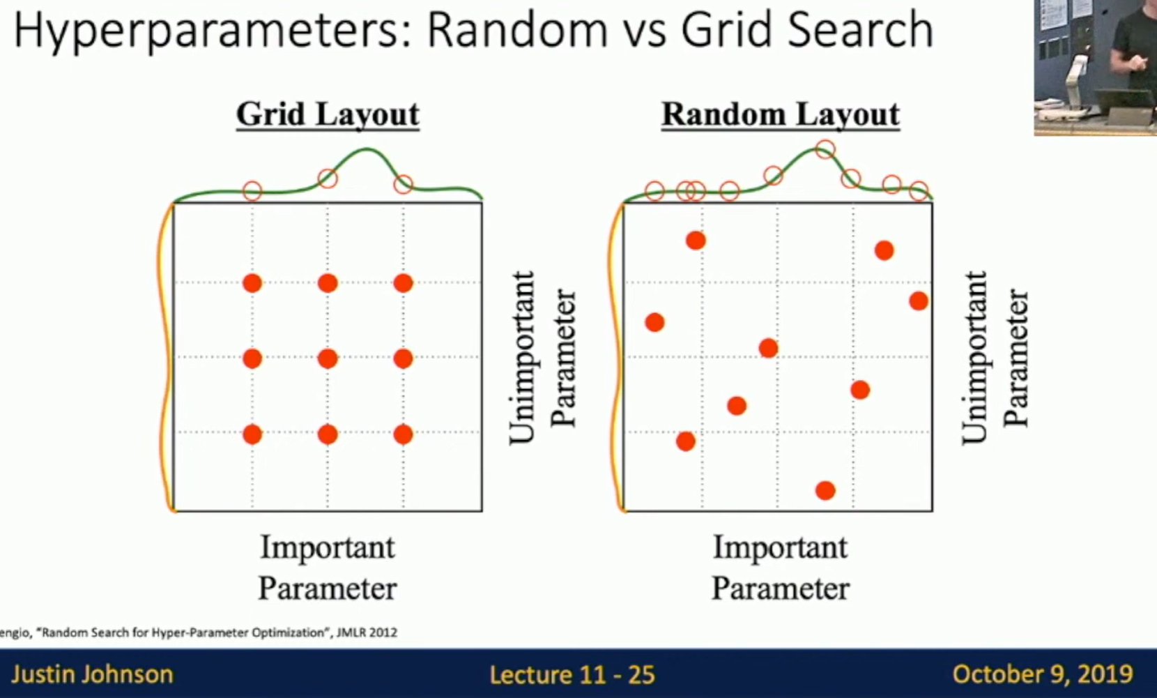
Fig: Random search

Experiment: Hyperparameters are often correlated.

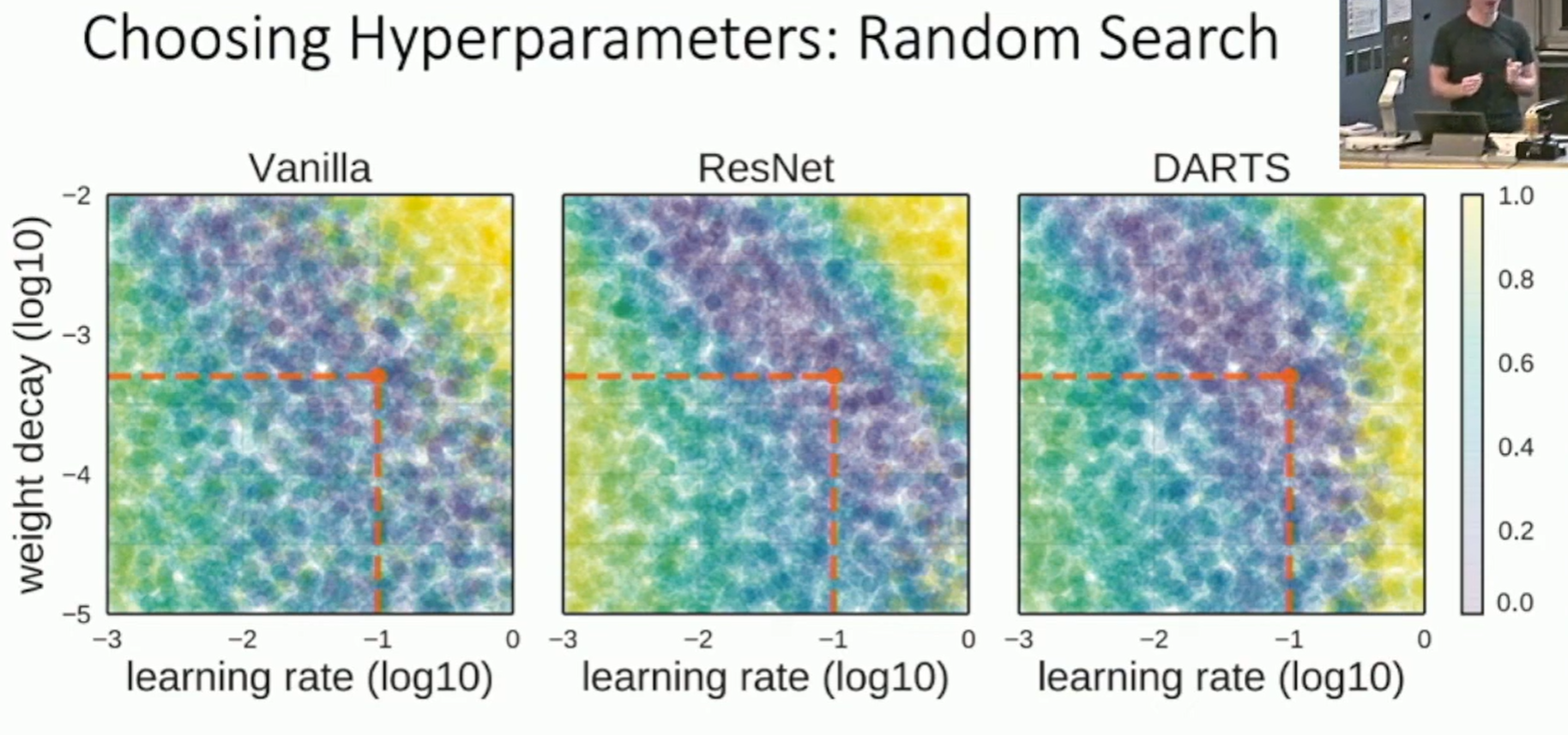
Fig: Experiment

When resources are limited

Step 1. Check initial loss

Turn off weight decay, sanity check loss at initialization. e.g. log(C) for softmax with C classes.

Step 2. Overfit a small sample

Try to train 100% training accuracy on a small sample. 5-10 mini-batches. Turn off all regularization. fiddle with(随意摆弄) architecture, learning rate, weight initialization, etc.

Loss not going down ? LR too low, bad initialization Loss explodes to Inf or NaN ? LR too low, bad initialization.

Step 3. Find LR that makes loss go down

Use the architecture from the previous step, use all training data, turn on small weight decay, find a learning rate that makes the loss drop quickly within 100 iterations.

Good learning rates to try: 1e-1, 1e-2, 1e-3, 1e-4.

Step 4. Coarse grid, train for 1~5 epochs

Choose a few values of learning rate and weight decay around what worked from Step 3, train a few models for 1~5 epochs.

Good weight decays to try: 1e-5, 1e-4, 0.

Step 5. Refine grid, train longer

Step 6. Look at learning curves, fine-tune

Losses may be noisy, use scatter plot to see the trend.

Examples

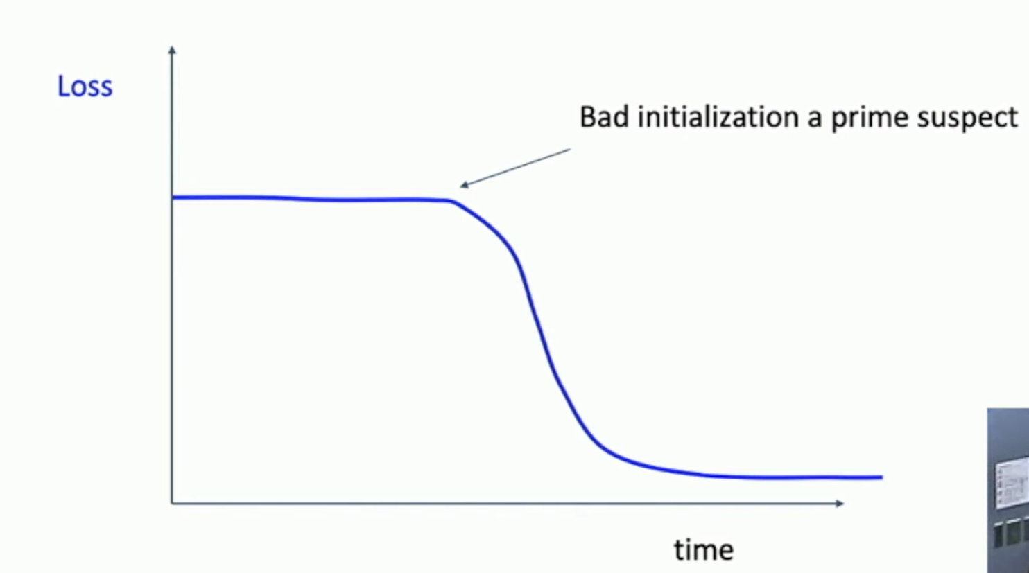
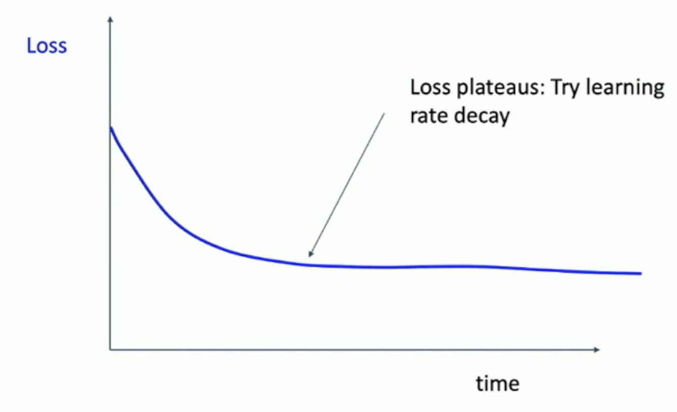
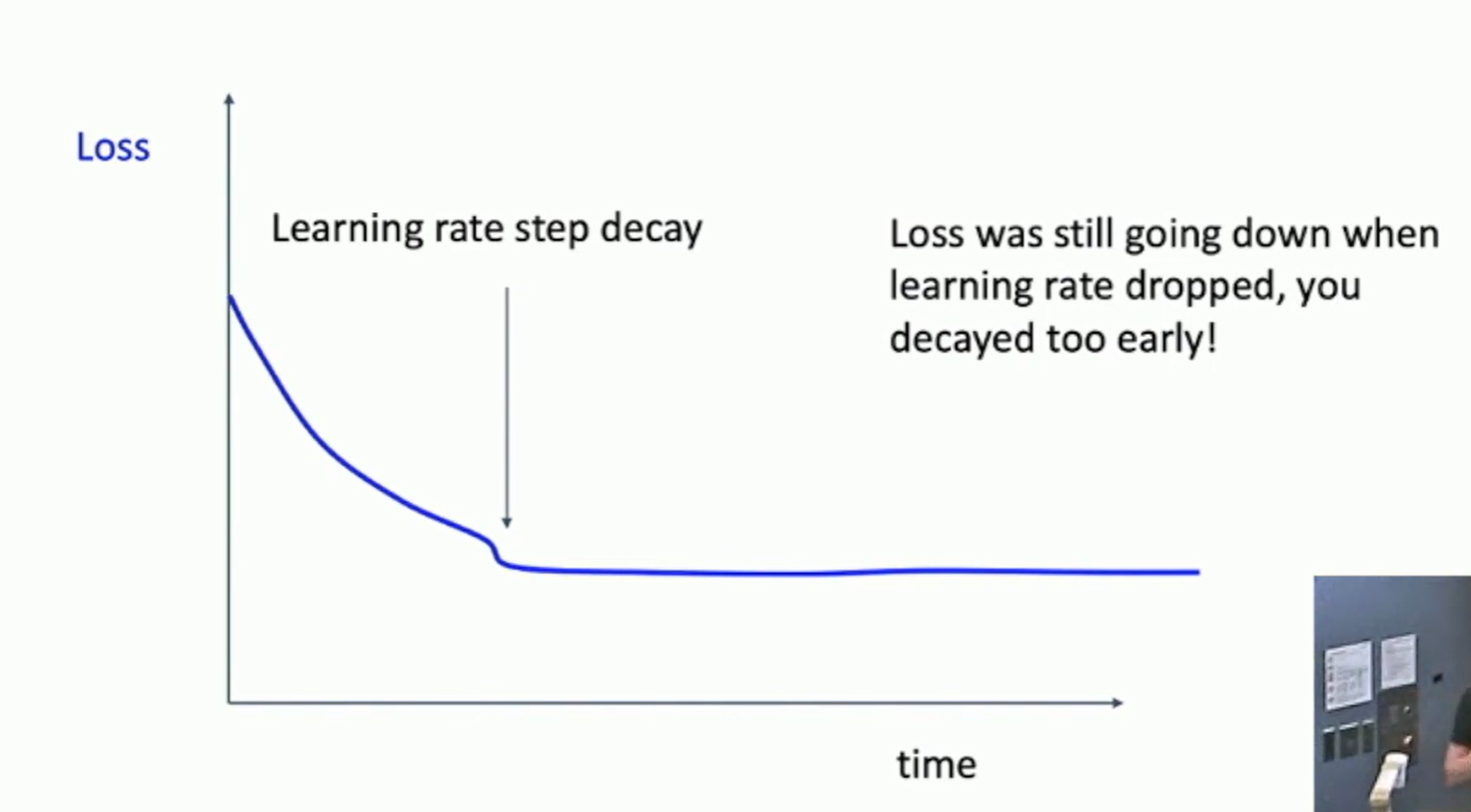
Fig: Learning curves

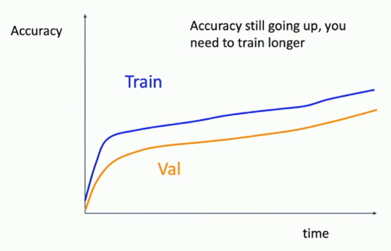
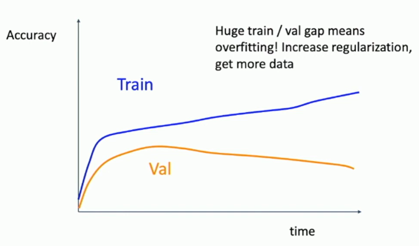
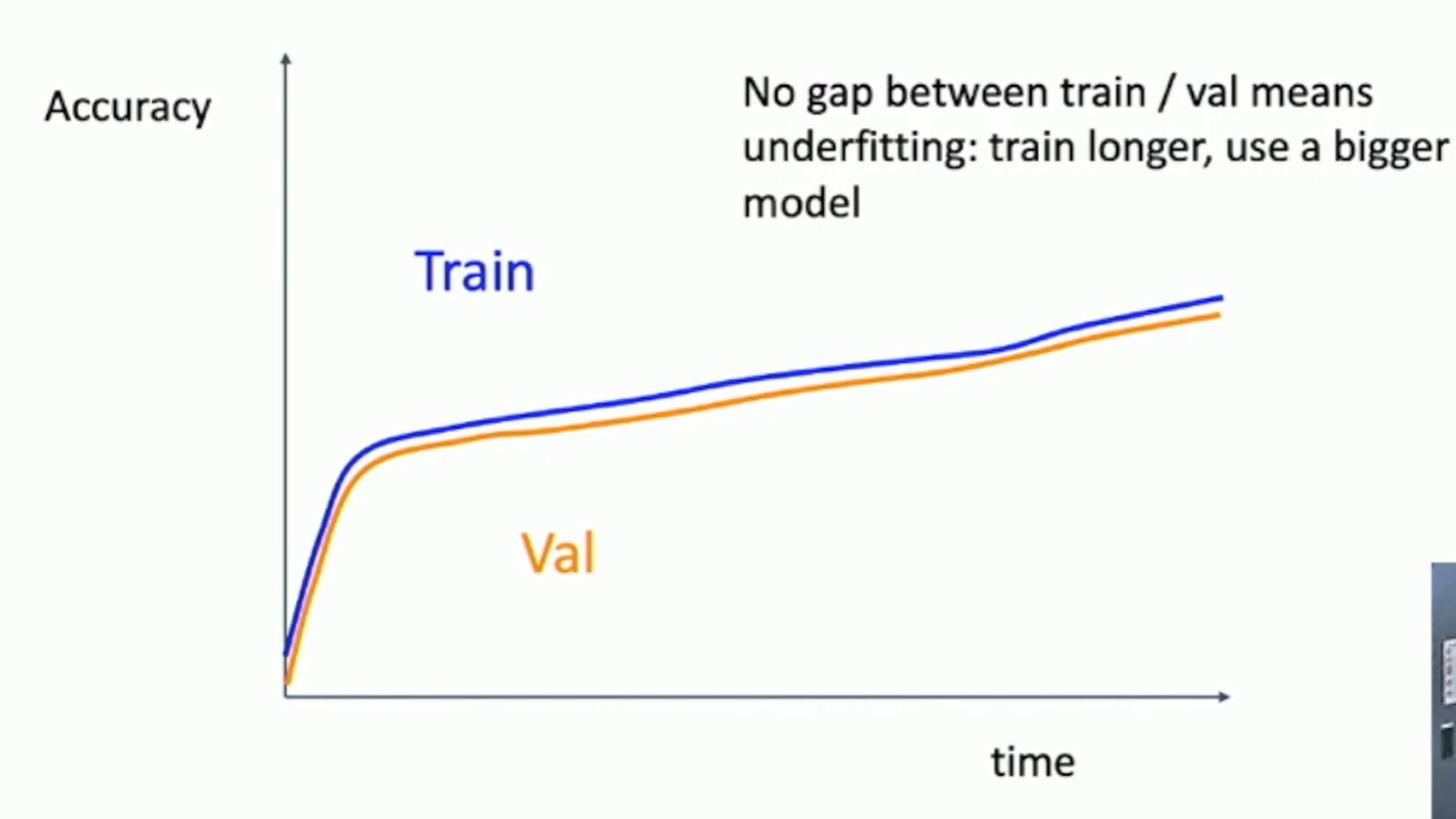
Fig: Learning curves

Step 7. GOTO Step 5

Tuning is like DJing. You need to keep adjusting the knobs until you get the right sound 🎶

TensorBoard

TensorBoard is a visualization tool that comes with TensorFlow. It allows you to visualize your training process.

Track ratio of weight update / weight magnitude

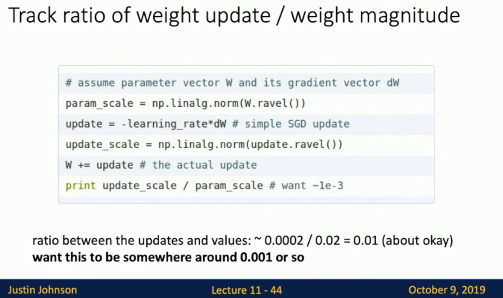
Fig: Track ratio of weight update / weight magnitude

After training

Model ensembles, transfer learning

Model ensembles

1. Train multiple independent models
2. At test time, average their predictions (Take average of predicted probability distributions, then choose argmax)

~ Enjoy 2% extra performance

Tips and tricks:

• Saving multiple checkpoints during training may also be a method of ensembling.
• Keeps tracking the running average of the weights during training.
• Periodic learning rate decay

Transfer learning

"You need a lot of data if want to train/use CNNs"

Transfer Learning with CNNs

1. Train on ImageNet
2. Remove the last FC
3. Use CNN as a feature extractor, freeze the weights of the CNN

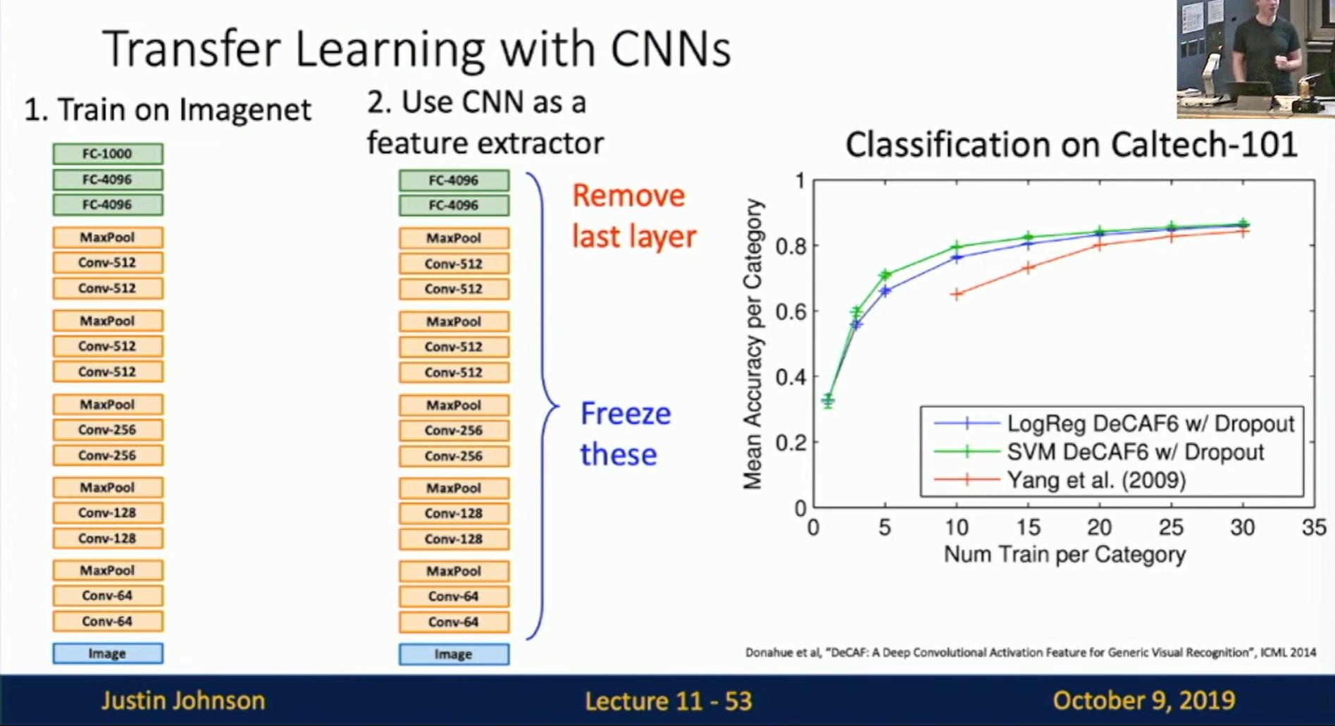
Fig: Transfer Learning with CNNs

4. Bigger dataset: Fine-Tuning. Continue training the entire model for a new task.

Some tricks:

• Train with feature extraction first before fine-tuning.
• Lower the learning rate: use ~1/10 of LR used in original training.
• Sometimes freeze lower layers to save computation.

Architecture Matters!

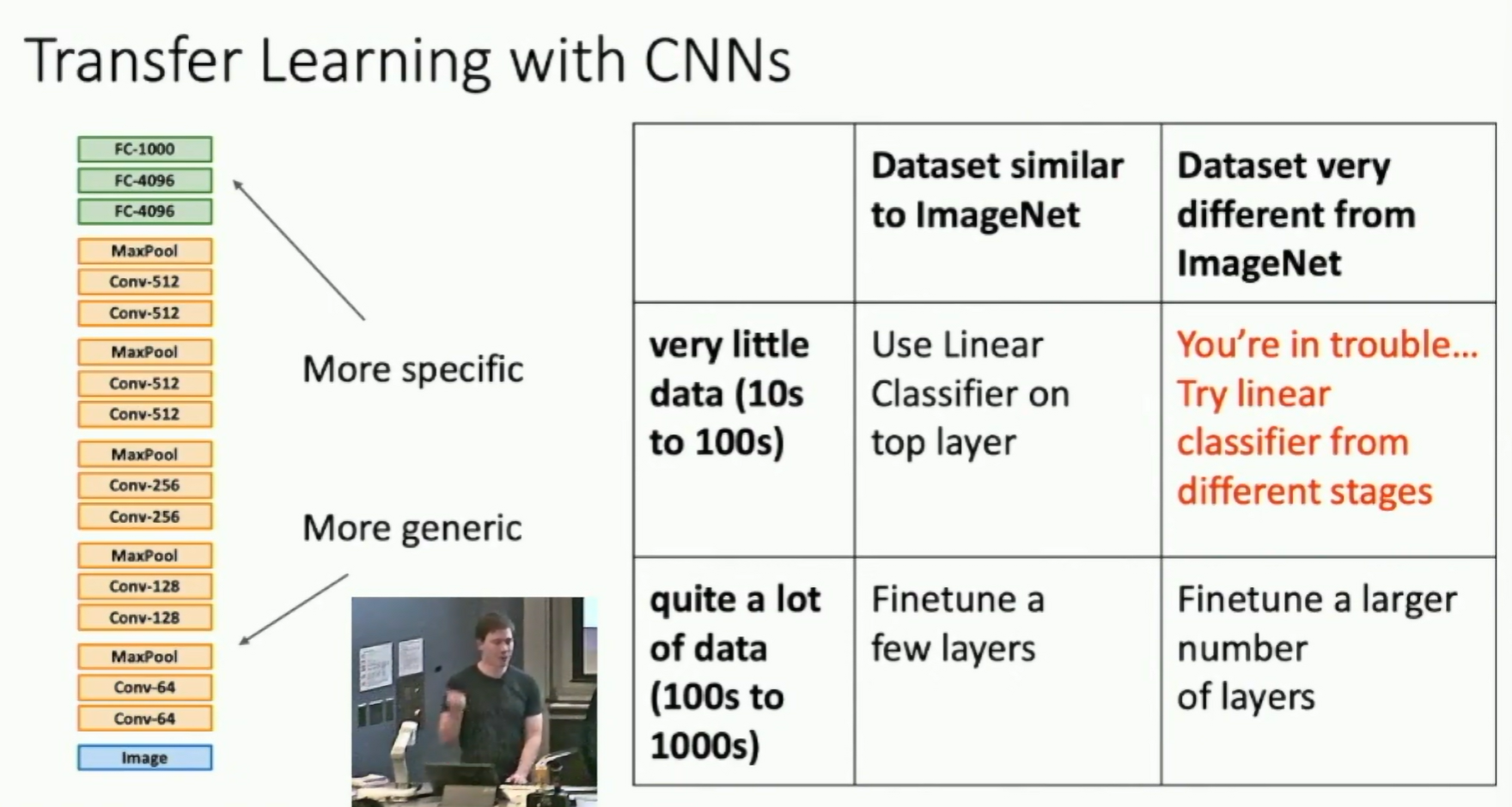
Fig: Transfer Learning with CNNs

Transfer learning is pervasive!

It's the norm, not the exception

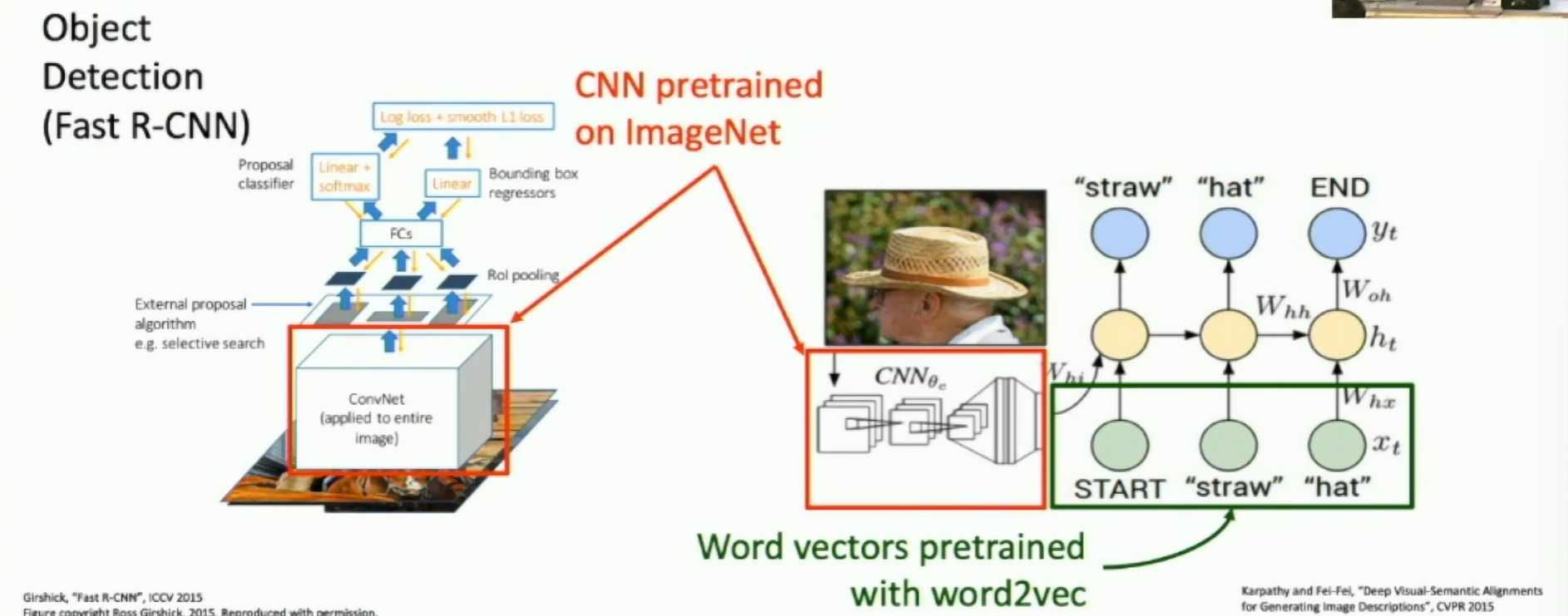
Fig: Transfer learning is pervasive

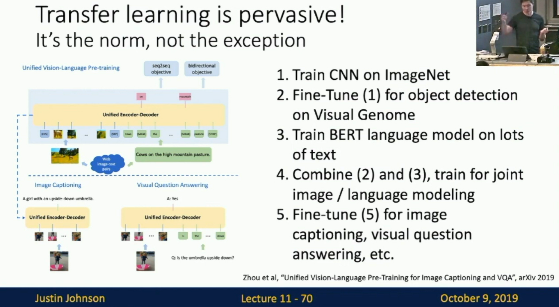
Fig: Transfer learning is pervasive

Pretraining - Transfer learning - Fine-tuning has become the norm.

Some very recent results have questioned it

Is this really critical?

Training from scratch can work as well as pretraining on ImageNet! ... If you train 3x as long

See Rethinking ImageNet Pre-training

Lots of work left to be done...

Large batch training

Scale the learning rate

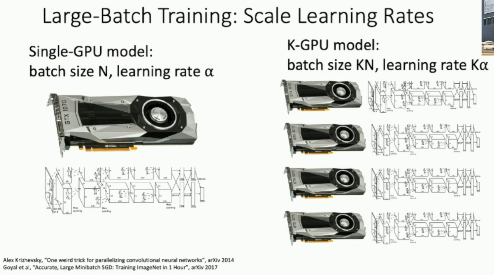
Fig: Large batch training

Learning Rate Warmup

Very large learning rate at the beginning may cause the model to diverge; linearly increasing learning rate from 0 over the first ~5000 iterations can prevent this.

Other Concerns:

Be careful with weight decay, batch normalization, and data shuffling.

For batch normalization, only normalize within a GPU.

Training ImageNet in 1 hour

batch size = 8192, 256 GPUs

... and now we achieved several minutes to train ImageNet

Notice on Usage and Attribution

This note is based on the University of Michigan's publicly available course EECS 498.008 / 598.008 and is intended solely for personal learning and academic discussion, with no commercial use.

• Nature of the Notes: These notes include extensive references and citations from course materials to ensure clarity and completeness. However, they are presented as personal interpretations and summaries, not as substitutes for the original course content.
• Original Course Resources: Please refer to the official University of Michigan website for complete and accurate course materials.
• Third-Party Open Access Content: This note may reference Open Access (OA) papers or resources cited within the course materials. These materials are used under their original Open Access licenses (e.g., CC BY, CC BY-SA).
• Proper Attribution: Every referenced OA resource is appropriately cited, including the author, publication title, source link, and license type.
• Copyright Notice: All rights to third-party content remain with their respective authors or publishers.
• Content Removal: If you believe any content infringes on your copyright, please contact me, and I will promptly remove the content in question.

Thanks to the University of Michigan and the contributors to the course for their openness and dedication to accessible education.