@Credits: EECS 498.007

Personal work for the assignments of the course: github repo.

Linear Classifiers：Parametric Approach

General form of a parametric classifier

Image $x$ -> $f(x,W)$ -> $y$ prediction

Example: $f(x,W)=Wx+b$

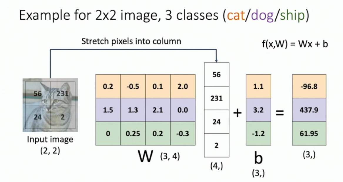
Fig: Linear classifier with 3 classes

• Preditions are linear when ignoring the bias term.

Visual Viewpoint

• Linear classifiers has one "template" per category. We take the dot product of the template with the image, and the highest dot product wins.
• Since each category only has one template, the decision ability is relatively limited. e.g. horse template has two heads!

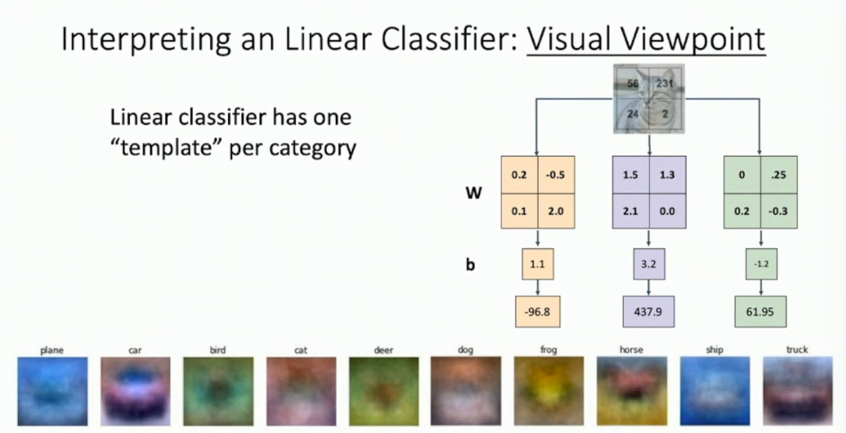
Fig: Visual Viewpoint

Geometric Viewpoint

• The decision boundary is a hyperplane. (Each row of the matrix is a covector)

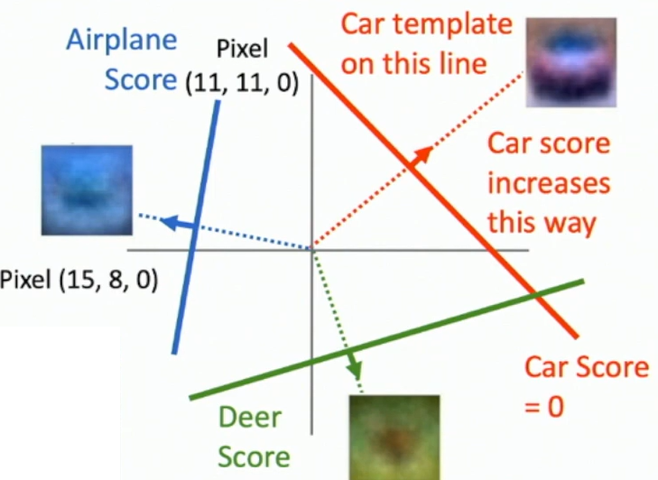
Fig: Decision hyperplanes

• It could be hard for the linear classifier to separate the classes if they are not linearly separable.

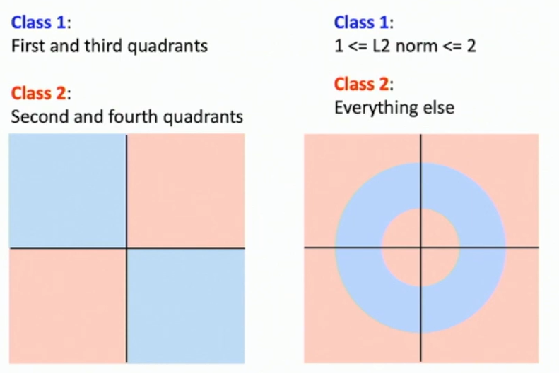
Fig: Hard cases

Recall: Perceptrons cannot learn XOR function!

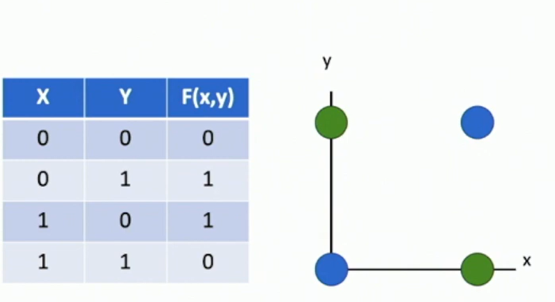
Fig: XOR logic

Loss: quantify how good a value $W$ is

Intuition: low loss = good classifier, high loss = bad classifier

Given a dataset of $N$ examples, $\{(x_i,y_i)\}_{i=1}^N$, where $x_i$ is the image and $y_i$ is the (integer) label.

Loss for a sing example: $L_i(f(x_i,W),y_i)$

Loss for the dataset: $L(W) = \frac{1}{N} \sum_{i=1}^N L_i(f(x_i,W),y_i)$

Multiclass SVM Loss

$$L_i(f(x_i,W),y_i) = \sum_{j\neq y_i} \max(0, s_j - s_{y_i} + 1)$$

• If $s_j$ is less than $s_{y_i}$ is by at least 1, then its contribution to the loss is 0.
• otherwise, it contributes to the loss by the difference between the scores plus 1.

Q: What happens to the loss if the score for the car image change a bit? A: Zero loss is still achieved if the input changes a bit.

Q2: min and max loss? A: min = 0, max = $\infty$ (if the score for the correct class is way less than the score for the incorrect class)

Q3: If all the score were random, what loss would we expect? A: The expected score of the correct and incorrect class would be approximately the same, sothe the loss would be around $C-1$, where $C$ is the number of classes. (小技巧：This is a good debugging technique to see if the initializations are corrects)

Q4: What would happen if the sum were over all classes? A: All the loss will be inflated by 1 but we will not change the ranking of the scores.

Q5: What if we use the mean instead of the sum? A: The loss will be the same but the gradient will be scaled by $\frac{1}{N}$. Its behavior is equivalent to the sum of the loss.

Q6: What if we used the square of the difference instead of the absolute value?

$L_i=\sum_{j\neq y_i} \max(0, s_j - s_{y_i} + 1)^2$

Q7: Suppose we found some $W$ with $L(W)=0$. Is it unique? No, we can scale $W$ by any constant greater than 1 and the loss will still be 0.

Regularization: Beyond Training Error

$$L(W) = \frac{1}{N} \sum_{i=1}^N L_i(f(x_i,W),y_i) + \underbrace{\lambda R(W)}_{\text{Regularization term}}$$

where $\lambda$ is a hyperparameter call the regularization strength.

Other regularizers: L2, L1, Droutout, Batch Normalization, etc.

Purpose of regularization:

• express preferencess in among models beyond "minimize training error"
• prefer simple models, prevent overfitting
• improve optimization by adding curvature

L1 regularization: This loss likes to "sparsify" the weights, to put weights to several dimensions.

L2 regularization: This loss likes to "spread out" the weights.

Cross-entropy loss

We can interpret raw classifier scores as probabilities.

$$s = f(x_i,W) \quad \hat P(Y=k|X=x_i) = \text{softmax}(s) = \frac{e^{s_{y_i}}}{\sum_j e^{s_j}}$$

$$L_i = -\log \hat P(Y=y_i|X=x_i) = -\log \left(\frac{e^{s_{y_i}}}{\sum_j e^{s_j}}\right)$$

Q: What is the minimum and maximum loss $L_i$ ?

A: min = $0$, max = $\infty$, and the loss is zero only if the prediction is a one-hot vector.

Q: If all scores are random, what loss would we expect? A: -log(1/C)=log(C), where C is the number of classes. (log(10)=2.3)

Optimization

$$W^*= \arg \min_W L(W)$$

Gradient Descent

$$W \leftarrow W - \alpha \nabla_W L(W)$$

where $\alpha$ is the learning rate.

Computing the gradient

Numeric gradient:

torch.autograd.gradcheck calculates the numerical gradient and compares it to the analytical gradient.

torch.autogrd.gradgradcheck calculates the numerical gradient of the gradient (Hessian) and compares it to the analytical gradient of the gradient.

Hyperparameters:

• weight initializations
• number of iterations
• learning rate

Batch Gradient Descent

Full gradient descent: compute the gradient of the loss with respect to the weights for the entire dataset.

$$L(W) = \frac{1}{N} \sum_{i=1}^N L_i(f(x_i,W),y_i)$$

$$W \leftarrow W - \alpha \nabla_W L(W) = W - \alpha \frac{1}{N} \sum_{i=1}^N \nabla_W L_i(W)$$

Schocastic gradient descent: compute the gradient of the loss with respect to the weights by drawing small subsamples.

Fig: Stochastic gradient descent

Problems with SGD:

• Loss changes quickly in one direction
• Saddle points

Variants of SGD

Momentum

$$v \leftarrow \beta v - \alpha \nabla_W L(W)$$

$$W \leftarrow W + v$$

where $\beta$ is the momentum term.

Nesterov momentum

$$v \leftarrow \beta v - \alpha \nabla_W L(W + \beta v)$$

$$W \leftarrow W + v$$

"Look ahead" before computing the gradient; computing the gradient there and mix it with velocity to get actual update direction.

AdaGrad

$$G \leftarrow G + \nabla_W L(W) \odot \nabla_W L(W)$$

where $\odot$ is element-wise multiplication.

$$W \leftarrow W - \alpha \nabla_W L(W) \oslash \sqrt{G + \epsilon}$$

where $\oslash$ is element-wise division, and $\epsilon$ is a small constant to prevent division by zero, e.g. $10^{-8}$.

Idea: adapt the learning rate for each parameter based on the history of the gradients: if the gradient is large, then the learning rate is small.

Problem: $G$ will keep increasing, and the learning rate will keep decaying.

RMSProp: Leaky AdaGrad

$$G \leftarrow \beta G + (1-\beta) \nabla_W L(W) \odot \nabla_W L(W)$$

$$W \leftarrow W - \alpha \nabla_W L(W) \oslash \sqrt{G + \epsilon}$$

where $\beta$ is a decay rate.

Adam: RMSProp with momentum

$$m \leftarrow \beta_1 m + (1-\beta_1) \nabla_W L(W)$$

$$v \leftarrow \beta_2 v + (1-\beta_2) \nabla_W L(W) \odot \nabla_W L(W)$$

$$W \leftarrow W - \alpha \frac{m}{\sqrt{v} + \epsilon}$$

where $\beta_1$ and $\beta_2$ are decay rates.

Problem: At the beginning, the momentum term is small, and the learning rate is small, so the learning rate is too large.

Improvement: Bias correction

$$m \leftarrow \beta_1 m + (1-\beta_1) \nabla_W L(W)$$

$$v \leftarrow \beta_2 v + (1-\beta_2) \nabla_W L(W) \odot \nabla_W L(W)$$

$$\hat m = \frac{m}{1-\beta_1^t}$$

$$\hat v = \frac{v}{1-\beta_2^t}$$

$$W \leftarrow W - \alpha \frac{\hat m}{\sqrt{\hat v} + \epsilon}$$

where $t$ is the iteration number.

Adam with $\beta_1=0.9$, $\beta_2=0.999$, and $lr=1e-3,5e-4,1e-4$ is a good default.

Summary

Algorithm	Tracks first Algorithm moments (Momentum)	Tracks second moments (Adaptive learning rates)	Leaky second moments	Bias correction for moment estimates
SGD	×	×	×	×
SGD+Momentum	√	×	×	×
Nesterov	√	×	×	×
AdaGrad	√	√	×	×
RMSProp	√	√	√	×
Adam	√	√	√	√

Adam is a good default optimizer for most problems. SGD+Momentum can outperform Adam but may require more tuning.

If you can afford to do full batch updates then try out L-BFGS.(and don't forget to disable all sources of noise)

Second-order optimization:

Newton's method, BFGS, L-BFGS

Second-Order Taylor Expansion:

$$f(x) \approx f(x_0) + \nabla f(x_0)^T(x-x_0) + \frac{1}{2}(x-x_0)^T H(x-x_0)$$

The shape of the Hessian matrix is $D \times D$, where $D$ is the number of parameters, which is very expensive to compute. So second-order optimization is not widely used in deep learning.