Problem: All of the previous models flattens the input image into a vector. This loses the spatial structure of the image. CNNs are designed to work with image data directly.

@Credits: EECS 498.007 | Video Lecture: UM-CV 5 Neural Networks

Personal work for the assignments of the course: github repo.

Notice on Usage and Attribution

These are personal class notes based on the University of Michigan EECS 498.008 / 598.008 course. They are intended solely for personal learning and academic discussion, with no commercial use.

For detailed information, please refer to the complete notice at the end of this document

Components of CNN

• Convolutional Layers
• Pooling Layers
• Normalization Layers

Convolution Layer

Image: 3x32x32

Filter: 3x5x5 Convolve the filter with the image to get a dot product. The filter is convolved with the image by sliding it across the image. The output is a 1x28x28 map.

We have multiple (for example 6) filters, each filter produces a different output. The output of the convolutional layer is a stack of 6 (28x28) maps.

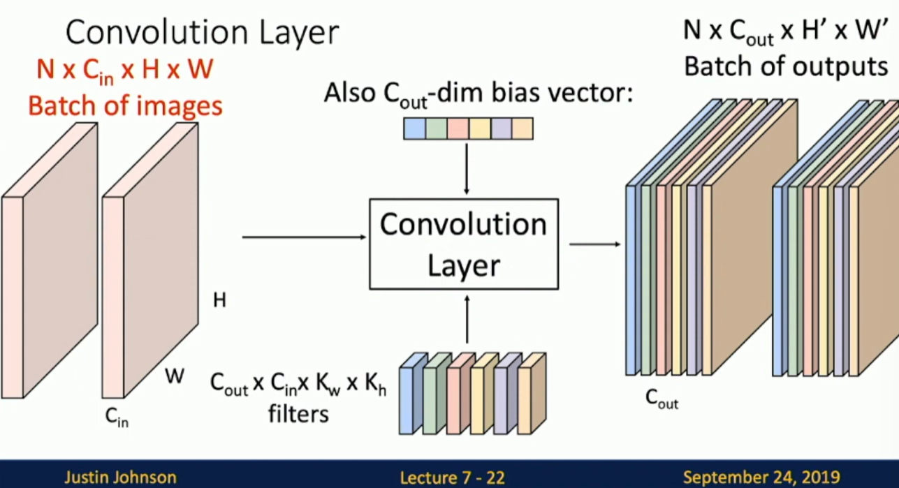
Fig: General form of convolutional layer

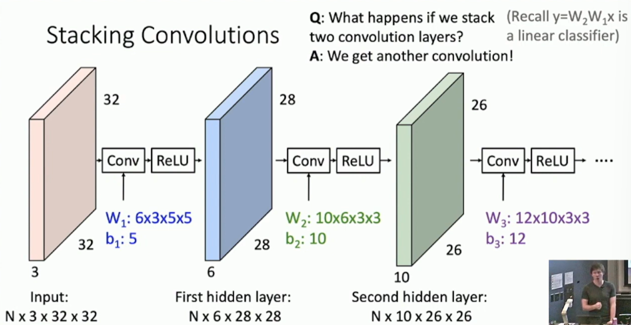
Fig: Stacking Convolutions

Typo: the length of $b_1$ is 6.

What do convolutional filters learn?

MLP: A set of template matching filters. Each filter is a set of weights that are learned during training. The filter is convolved with the input image to produce an output.

Convolutional Network: A set of local image templates, like edge detectors, corner detectors, etc.

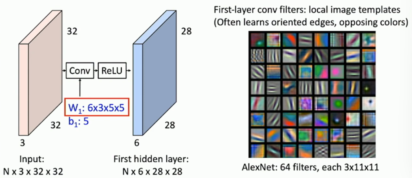
Fig: Convolutional Filters

Padding

A closer look at spatial dimensions

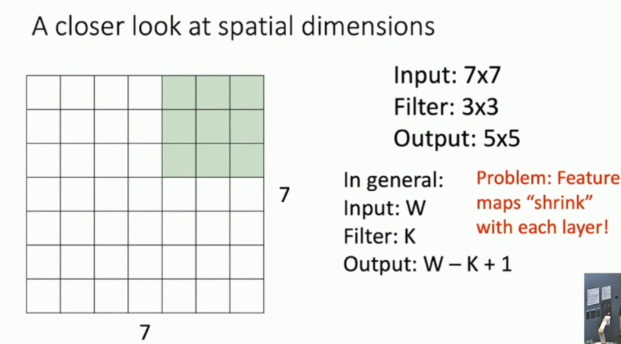
Fig: Convolutional Filters

Input: 7x7 -> Filter 3x3 -> Output: 5x5 In general: Input W -> Filter K -> Output W-K+1

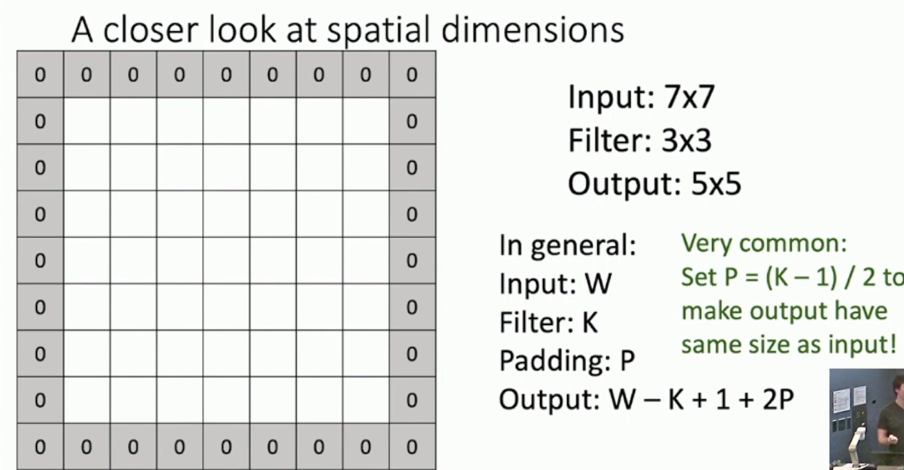
Fig: Padding

Receptive Field

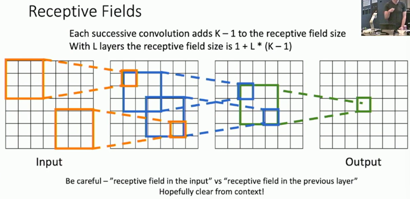
Fig: Receptive Field

The receptive field has two meanings: The kernel size and the field that the input dimension affects.

Strided Convolutions

Stride: The number of pixels the filter moves each time. Strided convolutions reduce the spatial dimensions of the output.

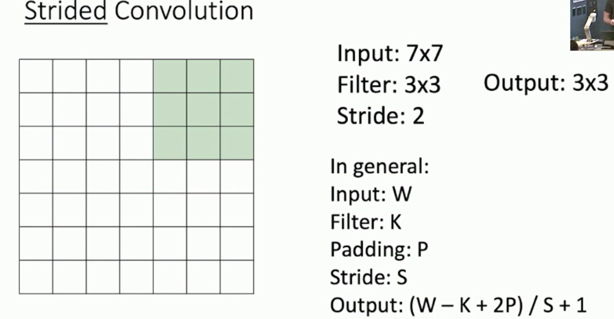
Fig: Strided Convolutions

Example:

Input volume 3x32x32 -> 10 3x5x5 filters with stride 1, padding 2 Output volume size? Number of parameters? Number of multiply-add operations?

Answer:
10x((32+4-5)/1+1)^2 = 10x32x32
10x3x5x5 + 10 = 760
768000, since each output pixel requires 3x5x5 multiplications. Total = 75 * (10*32*32) outputs = 768000

Example: 1x1 convolution

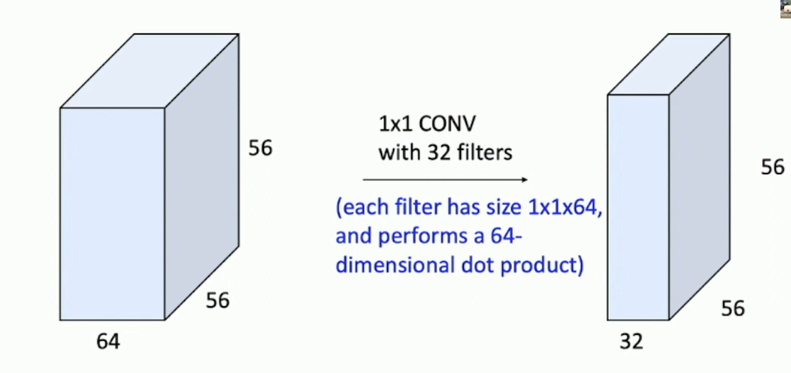
Fig: 1x1 Convolution

Stacking 1x1 convolution layers gives MLP operating on each input position. This preserves the spatial structure of the input.

Convolution Summary

• Input: C_in x H x W
• Hyperparameters: F filters, K kernel size, S stride, P padding
• Weight Matrix: C_out x C_in x K x K giving C_out filters of size KxK
• Bias vector: C_out
• Output: C_out x H_out x W_out
• H_out = (H + 2P - K)/S + 1
• W_out = (W + 2P - K)/S + 1

Other types of convolution

So far: 2D convolution. There are other types of convolutions like 1D, 3D, etc.

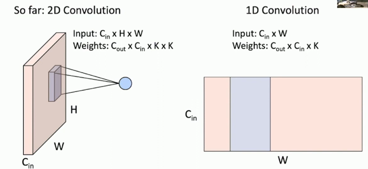
Fig: 1D Convolution

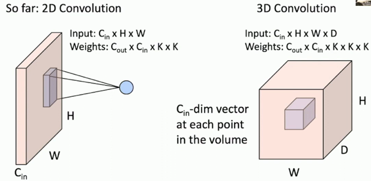
Fig: 3D Convolution

Pytorch has 1d to 3d convolutional layers.

Pooling Layer

The pooling layer is used to reduce the spatial dimensions of the input. It is used to reduce the number of parameters and computation in the network. It also helps in controlling overfitting.

Pooling is a form of downsampling. It reduces the spatial dimensions of the input.

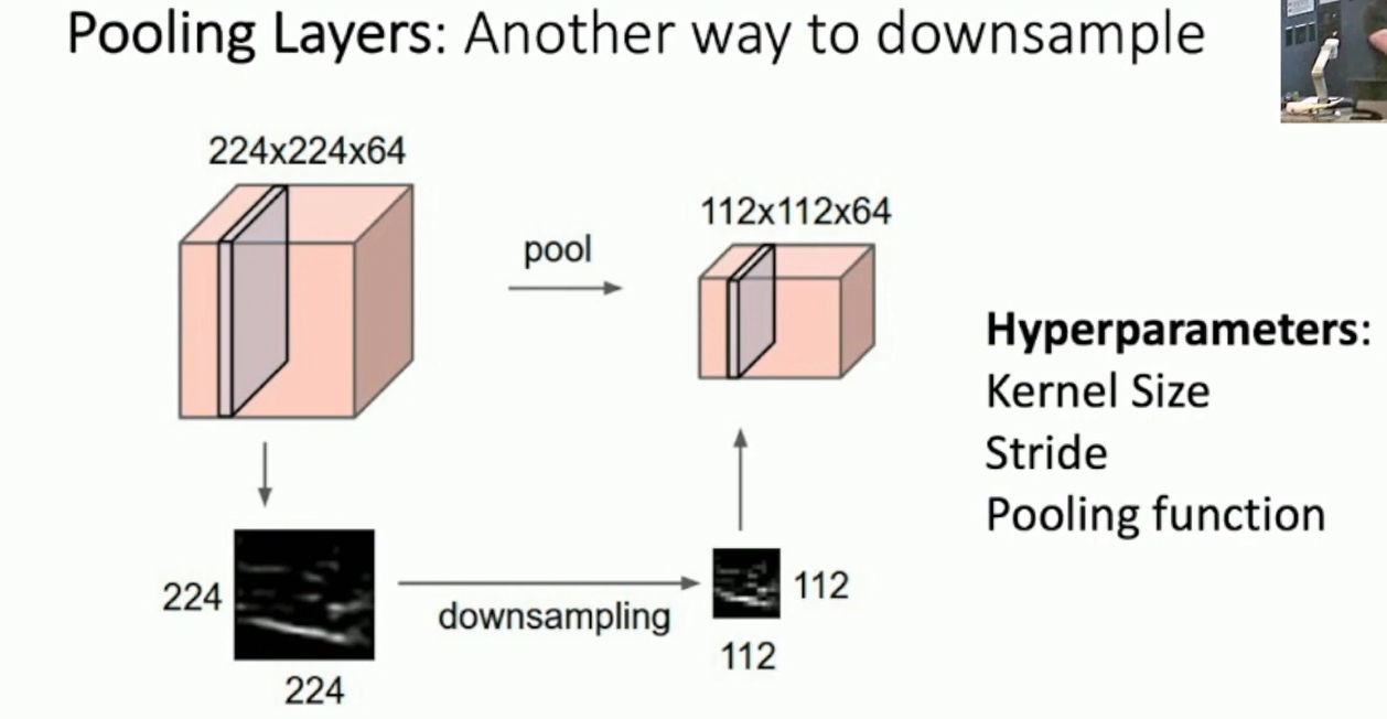
Fig: Pooling Layer

Types of pooling:

• Max pooling: Takes the maximum value in the pooling window.
• Average pooling: Takes the average value in the pooling window.

This introduces invariance to small spatial shifts, and there is no learnable parameters in pooling.

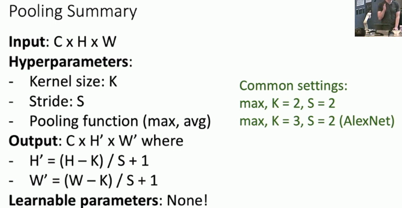
Fig: Pooling Summary

Convolutional Networks

Classic architecture:

Example: LeNet-5

Layer	Output Size	Weight Size
Input	1 x 28 x 28
Conv (C_out=20, K=5, P=2, S=1)	20 x 28 x 28	20 x 1 x 5 x 5
ReLU	20 x 28 x 28
MaxPool (K=2, S=2)	20 x 14 x 14
Conv (C_out=50, K=5, P=2, S=1)	50 x 14 x 14	50 x 20 x 5 x 5
ReLU	50 x 14 x 14
MaxPool (K=2, S=2)	50 x 7 x 7
Flatten	2450
Linear (2450->500)	50 x 7 x 7	2450 x 500
ReLU	500
Linear (500->10)	10	500 x 10

We tend to decrease the spatial dimensions and increase the number of channels as we go deeper into the network.

Training Deep Networks: Batch Normalization

Problem: Deep networks are hard to train. The gradients tend to vanish or explode as we go deeper into the network.

Solution: Batch Normalization

This helps reduce the internal covariate shift. It normalizes the activations of the network. It helps in training deeper networks.

(Joffe and Szegedy, ICML 2015, Batch Normalization: Accelerating Deep Network Training by Reducing Internal Covariate Shift)

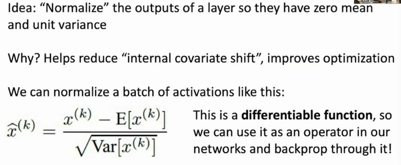
Fig: Batch Normalization

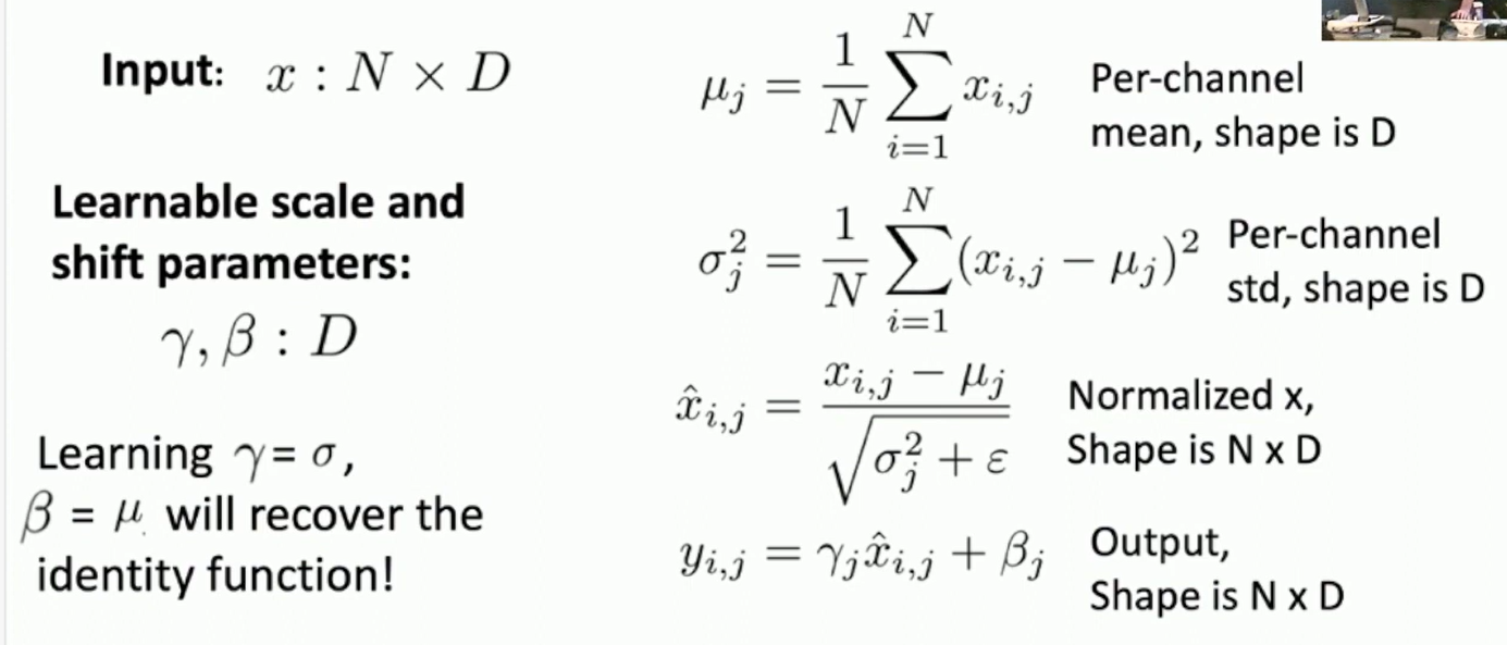
Fig: Calculating Batch Normalization

Calculating mean and variance over the batch means the inputs are intertangled. The estimation depends on the batch size.

During training, we use the batch mean and variance.

During testing, we use the average and variance of the entire seen data during training.

During testing, the batchnorm becomes a linear operator! We can fuse them into the previous layer.

Batch Normalization for Convolutional Networks

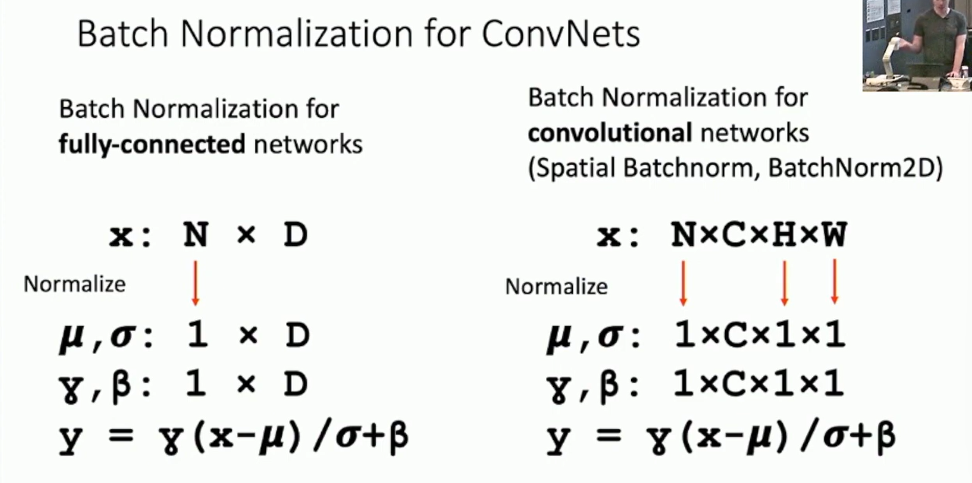
Fig: Batch Normalization for Convolutional Networks

See ICML 2015 paper for more details.

Advantages and Disadvantages of Batch Normalization:

• Makes deep networks much easier to train.

• Allows higher learning rates and faster convergence.

• Networks become more robust to initialization.

• Acts as regularization during training.

• Zero overhead at test time. Can be fused into the previous layer.

• Works well with feed-forward networks.

• Not well understood theoretically(yet)

• 0 Mean is forced, and may not be ideal for all models.

• Behaves differently during training and testing: this is a very common source of bugs!

Instance Normalization

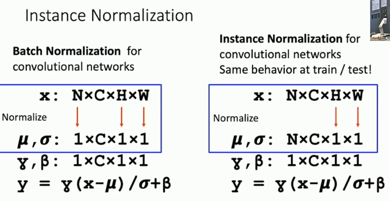
Fig: Instance Normalization

Fig: Different Normalization Techniques

CNN Architectures

ImageNet Classification Challenge

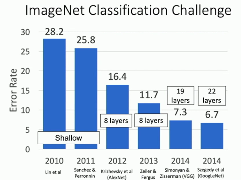
Fig: ImageNet Classification Challenge

AlexNet: 2012 winner. 8 layers, 60 million parameters.

227×227 inputs, 5 Convolutional layers, Max pooling, 3 Fully connected layers, ReLU nonlinearity. Used "local response normalization"(not used anymore). Trained on two GTX 580 GPUs - only 3GB of memory each. Model split over two GPUs.

Fun fact: citations to the AlexNet

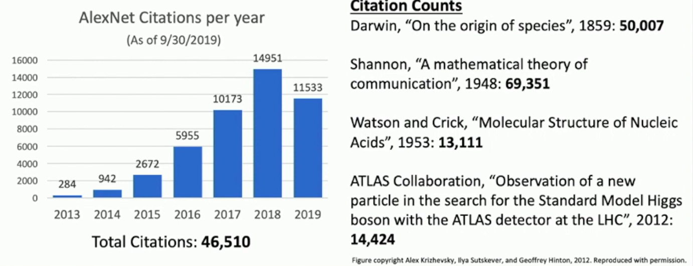
Fig: AlexNet

Layer	Input Size (C)	Input Size (H / W)	Filters	Kernel	Stride	Pad	Output Size (C)	Output Size (H / W)	Memory (KB)	Params (k)	FLOP (M)
conv1	3	227	64	11	4	2	64	56	784	23	73
pool1	64	56		3	2	0	64	27	182	0	0
conv2	64	27	192	5	1	2	192	27	547	307	224
pool2	192	27		3	2	0	192	13	127	0	0
conv3	192	13	384	3	1	1	384	13	254	664	112
conv4	384	13	256	3	1	1	256	13	169	885	145
conv5	256	13	256	3	1	1	256	13	169	590	100
pool5	256	13		3	2	0	256	6	36	0	0
flatten	256	6					9216		36	0	0
fc6	9216						4096		16	37,749	38
fc7	4096						4096		16	16,777	17
fc8	4096						1000		4	4,096	4

conv1: Number of floating point operations (multiply+add) = (number of output elements) * (ops per output element) = (64 * 56 * 56) * (11 * 11 * 3) = 72,855,552 = 73M flops

How is it designed? Trails and errors. Also a compromise between memory usage and computational efficiency.

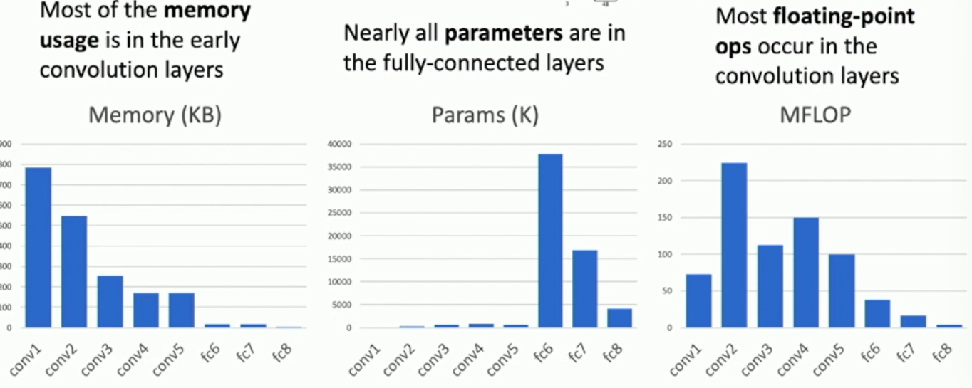
Fig: AlexNet

ZFNet: A Bigger AlexNet

Similar to AlexNet, but with smaller filters and deeper layers. 7x7 filters in the first layer, 3x3 filters in the second layer. Deeper layers.

VGG: The principles of designing a good network

• All conv are 3x3 stride 1 pad 1
• All max pool are 2x2 stride 2
  • Two convolutional layers together make a receptive field of 5x5, while having fewer parameters and less flops. We can also add ReLU after each layer to add non-linearity to the network.
• After pool, double the number of channels
  • We want each convolutional layer to have the same computational cost.
  • Input1: Cx2Hx2W - Conv(3x3, C->C) - 4HWC Memory - 9C^2 Params - 4HWC flops
  • Input2: 2CxHxW - Conv(3x3, 2C->2C) - 4HWC Memory - 36C^2 Params - 4HWC flops

5 stages: conv-conv-pool conv-conv-pool conv-conv-pool conv-conv-conv-(conv)-pool conv-conv-conv-(conv)-pool FC-FC-FC

VGG is much larger than AlexNet. It has 138 million parameters! VGG is 19.4x computationally more expensive than AlexNet.

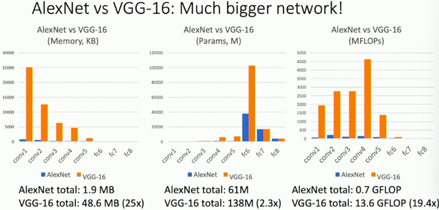
Fig: VGG

Done in academia by one grad and one faculty member.

Google LeNet: Focus on Efficiency

Design an efficient convolutional network for mobile devices. 22 layers, 4 million parameters.

Aggressive Stem downsamples the network at the beginning. 3x3 convolutions, 1x1 convolutions, and factorized convolutions. (CVPR 2015)

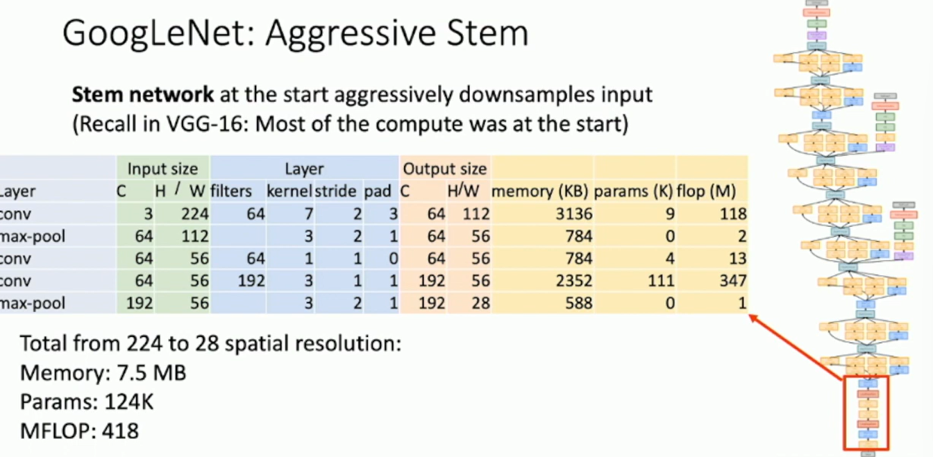
Fig: Google LeNet

Inception Module repeated throughout the network. It uses multiple filter sizes in parallel. It uses 1x1, 3x3, 5x5, and max pooling in parallel. It concatenates the outputs of these filters. Do all the kernel sizes in parallel and concatenate the outputs.

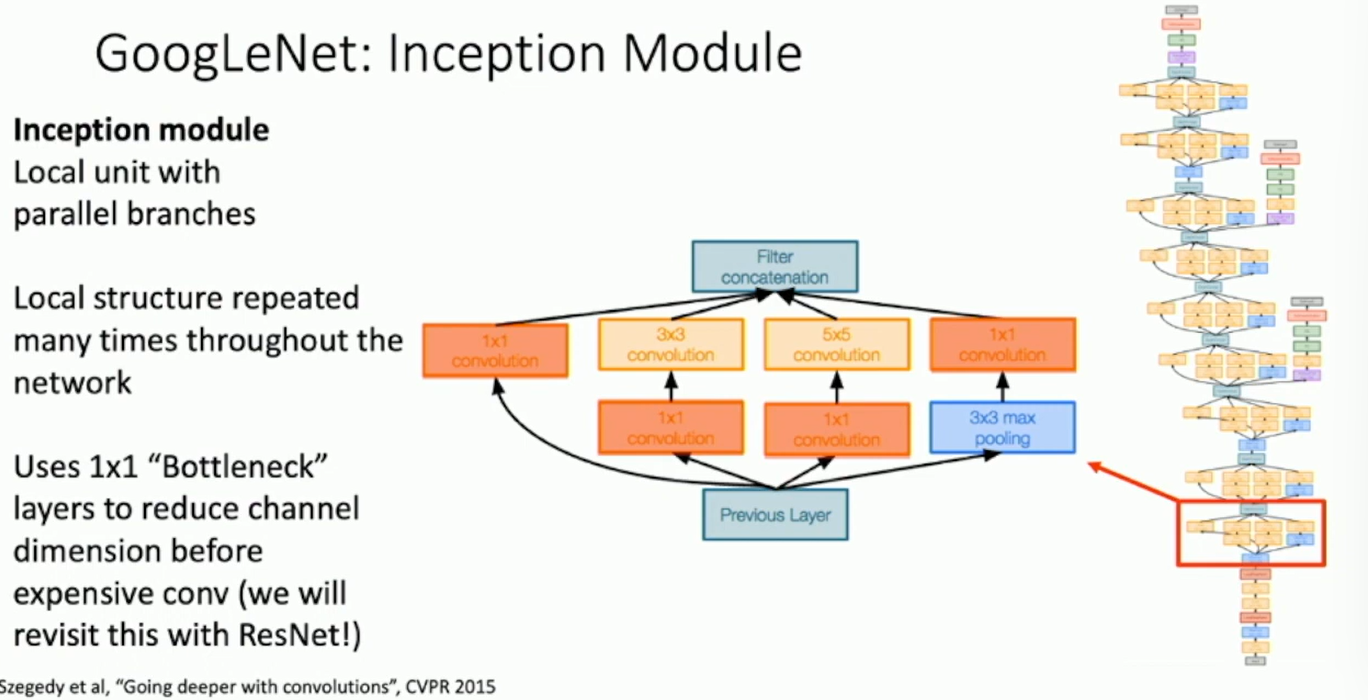
Fig: Inception Module

Global Average Pooling at the end. Rather than flatting tensor, it takes the average of the tensor.

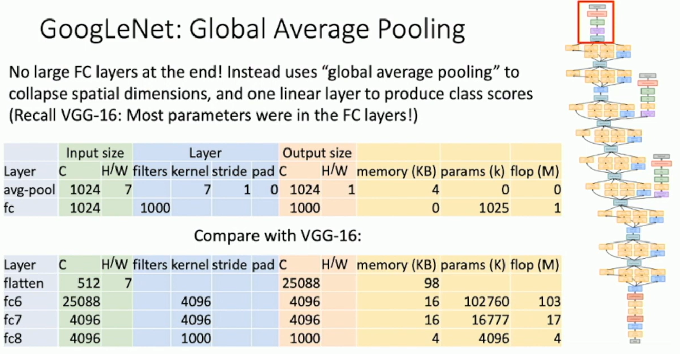
Fig: Global Average Pooling

Auxiliary Classifiers at intermediate layers. Making gradient flow easier. (For VGG, the network is trained layerwise.)

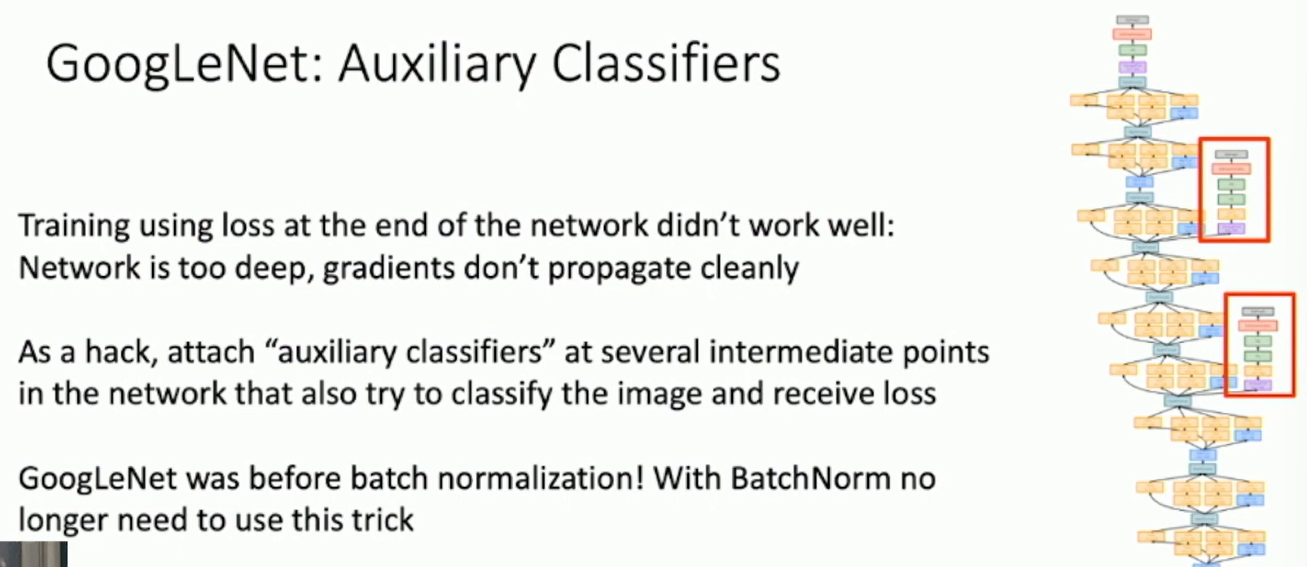
Fig: Auxiliary Classifiers

ResNet (CVPR 2016)

Deeper models does worse than shallow model!

Initial Guess: Deep model is overfitting. In fact, the training error of deeper networks is also higher than the shallower networks.

Hypothesis: This is an optimization problem. The deeper networks are harder to optimize, and in particular don't learn the identity functions to emulate the shallower networks.

Solution: Change the network so learning identity function is easier.

Residual Block: Instead of learning $H(x)$, learn $F(x) = H(x) - x$. The network learns the residual function.

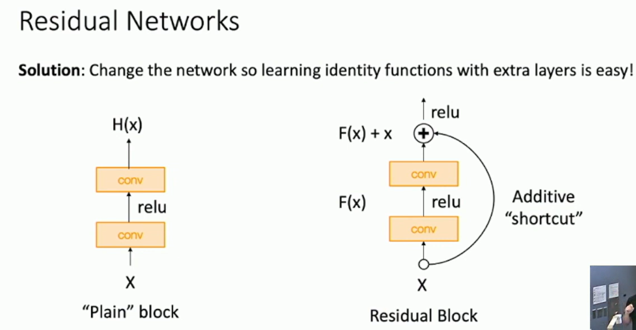
Fig: Residual Block

When backpropagating, the gradient is copied to the input. This makes the optimization easier.

Network is divided into stages like VGG. Each stage has a different number of filters.

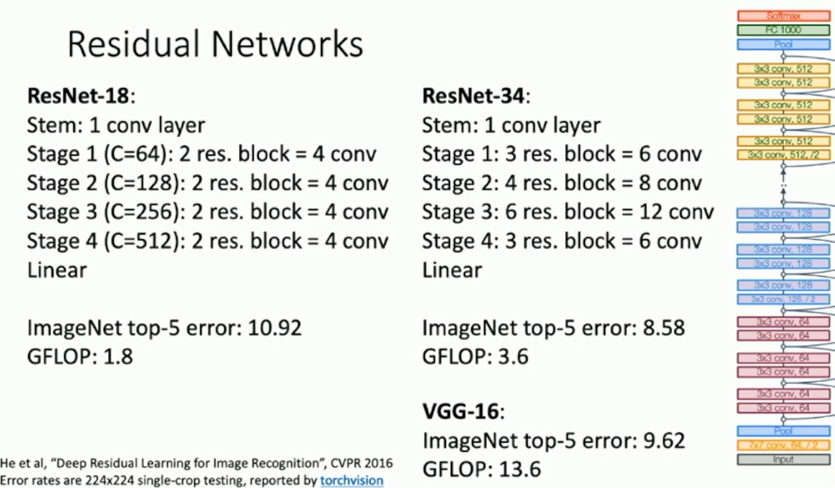
Fig: ResNet

Basic Block and Bottleneck Block

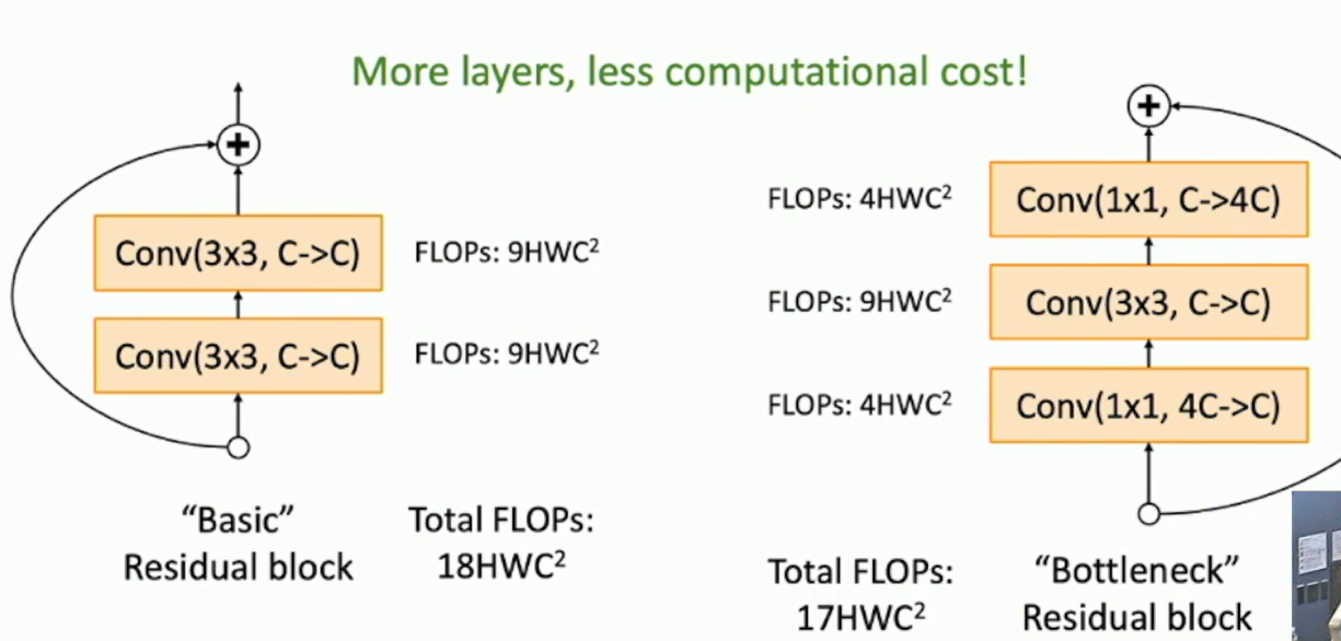
Fig: Basic Block and Bottleneck Block

In 2015, ResNet ranked 1st in all five competitions!

MSRA @ ILSVRC & COCO 2015 competitions

• ImageNet Classification
• ImageNet Detection
• ImageNet Localization
• COCO Detection
• COCO Segmentation

Comparing Complexity

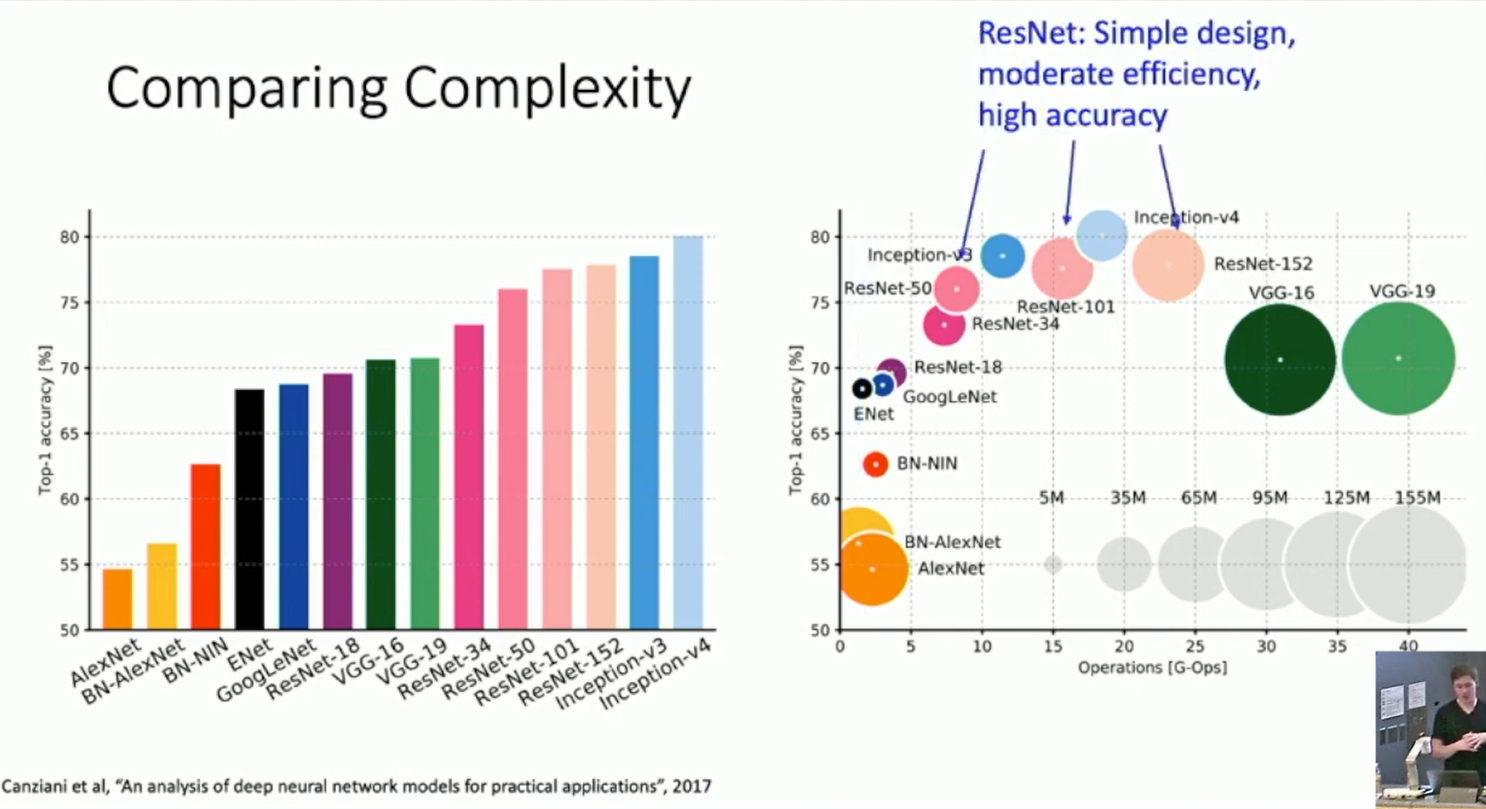
Fig: Comparing Complexity

ImageNet 2016 winner: Model Ensembles

ResNeXt

ResNeXt: Aggregated Residual Transformations for Deep Neural Networks (CVPR 2017)

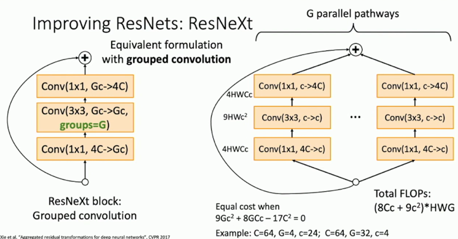
Fig: ResNeXt

Annual ImageNet competition is no longer held after 2017. Now it is moved to Kaggle as a challenge.

DenseNet

Densely Connected Convolutional Networks (CVPR 2017)

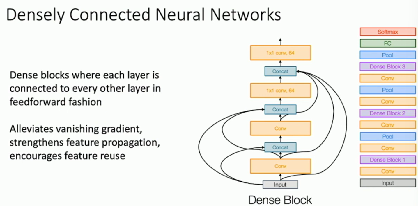
Fig: DenseNet

MobileNets: Tiny Networks

MobileNets: Efficient Convolutional Neural Networks for Mobile Vision Applications (CVPR 2017)

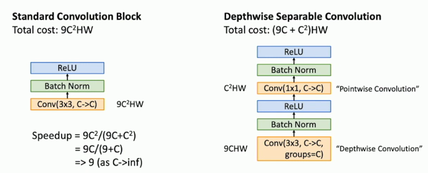
Fig: MobileNets

Also related:

ShuffleNet: An Extremely Efficient Convolutional Neural Network for Mobile Devices (CVPR 2018)

MobileNetV2: Inverted Residuals and Linear Bottlenecks (CVPR 2018)

ShuffleNetV2: Practical Guidelines for Efficient CNN Architecture Design (ECCV 2018)

Neural Architecture Search (NAS)

a hot topic in deep learning research

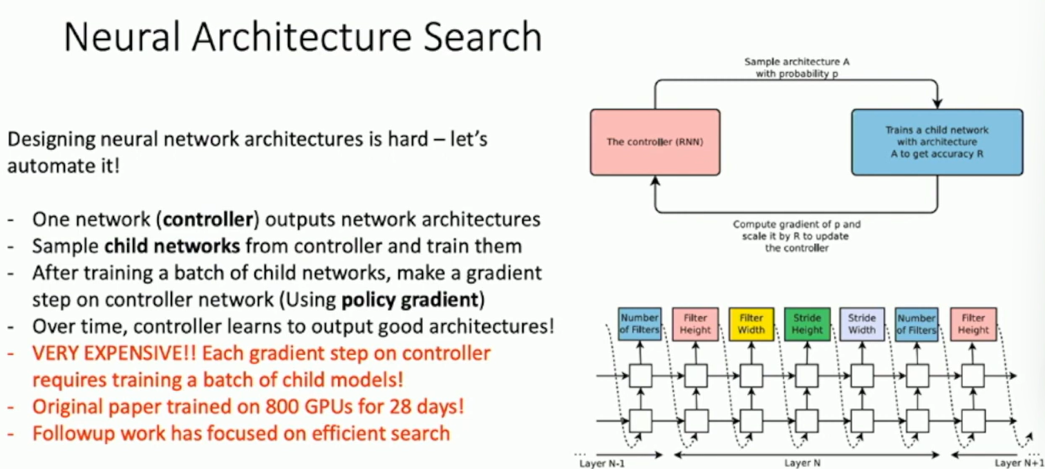
Fig: Neural Architecture Search

Summary

Early work (AlexNet, VGG) focused on designing deeper networks.

Later work (ResNet, DenseNet) focused on designing more efficient networks. Recent work (MobileNets, ShuffleNet) focused on designing networks for mobile devices.

Early work (AlexNet -> ZFNet -> VGG) shows that bigger networks work better

GoogLeNet one of the first to focus on efficiency (aggressive stem, 1x1 bottleneck convolutions, global avg pool instead of FC layers)

ResNet showed us how to train extremely deep networks - limited only by GPU memory! Started to show diminishing returns as networks got bigger

After ResNet: Efficient networks became central: how can we improve the accuracy without increasing the complexity?

Lots of tiny networks aimed at mobile devices: MobileNet, ShuffleNet, etc

Neural Architecture Search promises to automate architecture design

What architecture should I use?

For most problems you should use an off-the-shelf architecture (e.g. ResNet, DenseNet, etc)

If you just care about accuracy, ResNet-50 or ResNet-101 is a good choice.

If you care about efficiency, MobileNet or ShuffleNet is a good choice.

Notice on Usage and Attribution

This note is based on the University of Michigan's publicly available course EECS 498.008 / 598.008 and is intended solely for personal learning and academic discussion, with no commercial use.

• Nature of the Notes: These notes include extensive references and citations from course materials to ensure clarity and completeness. However, they are presented as personal interpretations and summaries, not as substitutes for the original course content.
• Original Course Resources: Please refer to the official University of Michigan website for complete and accurate course materials.
• Third-Party Open Access Content: This note may reference Open Access (OA) papers or resources cited within the course materials. These materials are used under their original Open Access licenses (e.g., CC BY, CC BY-SA).
• Proper Attribution: Every referenced OA resource is appropriately cited, including the author, publication title, source link, and license type.
• Copyright Notice: All rights to third-party content remain with their respective authors or publishers.
• Content Removal: If you believe any content infringes on your copyright, please contact me, and I will promptly remove the content in question.

Thanks to the University of Michigan and the contributors to the course for their openness and dedication to accessible education.