Summary: Deep learning hardware, software, and PyTorch modules.

@Credits: EECS 498.007 | Video Lecture: UM-CV 5 Neural Networks

Personal work for the assignments of the course: github repo.

Notice on Usage and Attribution

These are personal class notes based on the University of Michigan EECS 498.008 / 598.008 course. They are intended solely for personal learning and academic discussion, with no commercial use.

For detailed information, please refer to the complete notice at the end of this document

Heep Learning Hardware

GigaFLOPs per Dollar

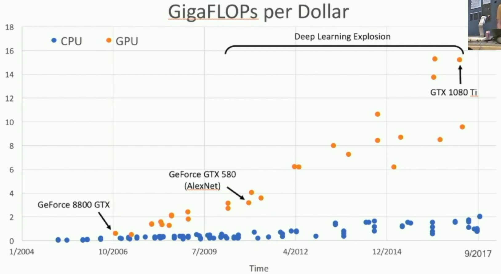
Fig: GigaFLOPS per Dollar

CPU: Fewer cores, but each core is much faster and much more capable; great at sequential tasks

GPU: More cores, but each core is much slower and "dumber"; great for parallel tasks

CPU vs GPU	Cores	Clock Speed (GHz)	Memory	Price	TFLOP/sec
CPU Ryzen 9 3950X	16 (32 threads with hyperthreading)	3.5 (4.7 boost)	System RAM	$749	~4.8 FP32
GPU NVIDIA Titan RTX	4608	1.35 (1.77 boost)	24 GB GDDR6	$2499	~16.3 FP32 ~130 with Tensor Cores

Inside a GPU

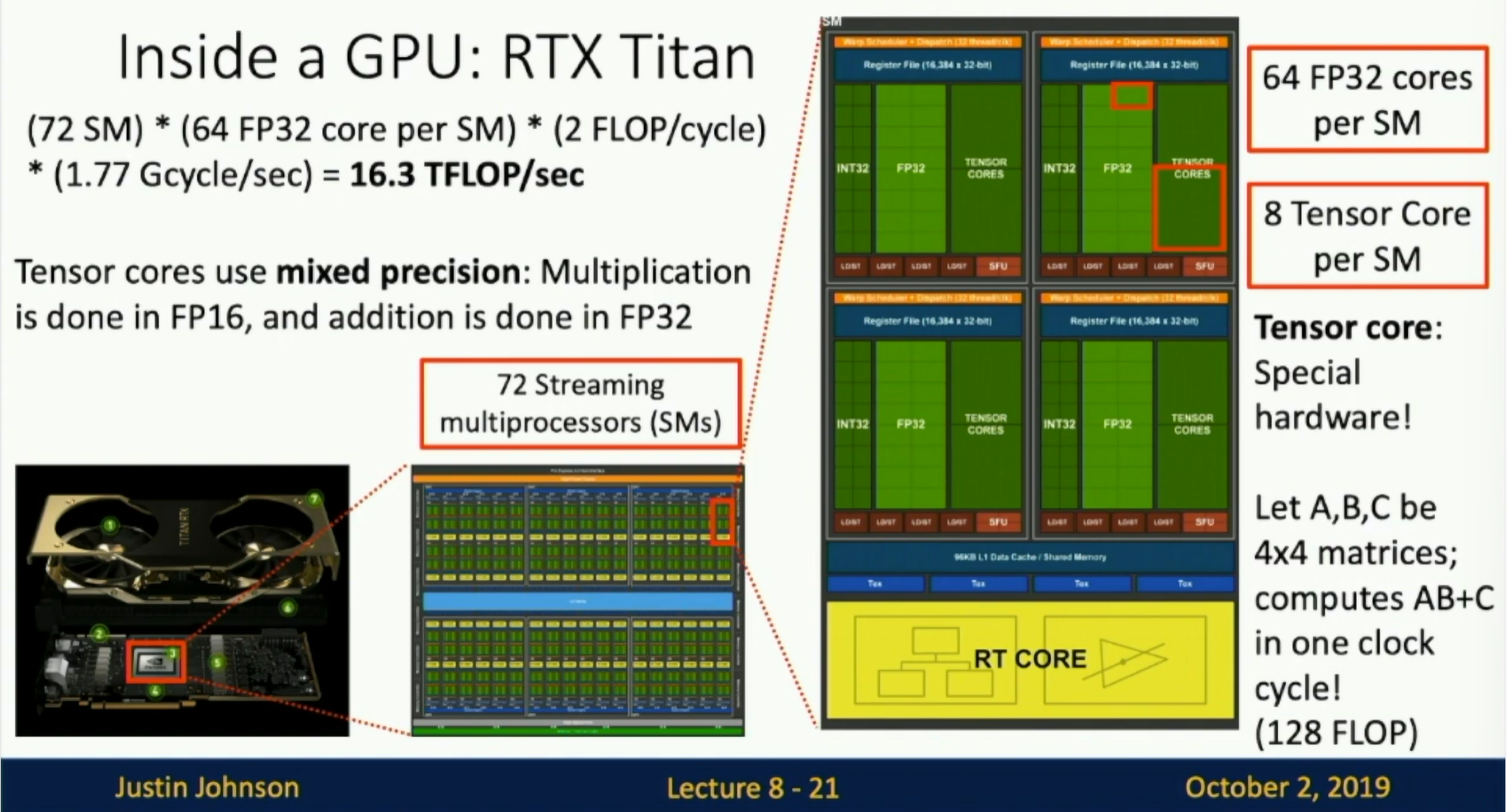
Fig: Inside a GPU

• 12 x 2GB memory modules
• 72 Streaming multiprocessors(SMs)
• Inside each SM:
  • 64 FP32 cores per SM
  • 8 Tensor Core per SM
    • Let A,B,C be 4x4 matrices This computes C = A x B + C in one clock cycle (128FLOP/cycle)
    • The multiplication is done in FP16
    • The accumulation is done in FP32
• 4608 FP32 cores in total
• 576 Tensor cores
• 72 SM x 64 cores x 2 FLOP /cycle x 1.77 GHz(Gcycle/sec) = 16.3 TFLOP/sec (FP32)
• 72 SM x 8 Tensor cores x 128 FLOP/cycle x 1.77 GHz(Gcycle/sec) = 130 TFLOP/sec (FP16)

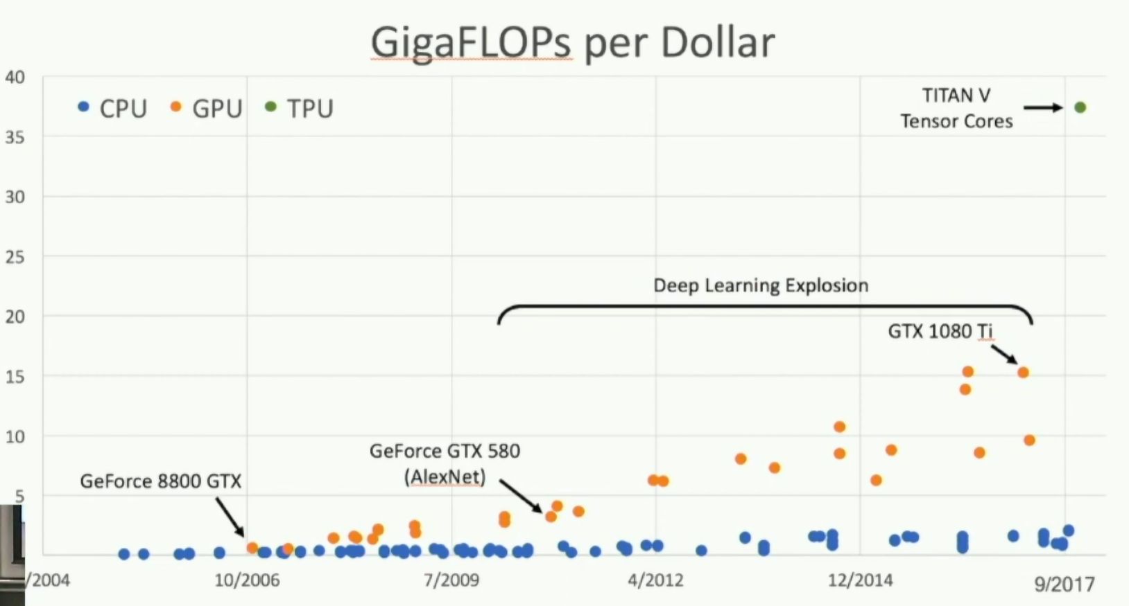
Fig: GigaFLOPs per dollar

How to utilize these cores? Store your tensor in FP16 and use the tensor cores for matrix multiplication.

Parallelism

Example: Matrix Multiplication

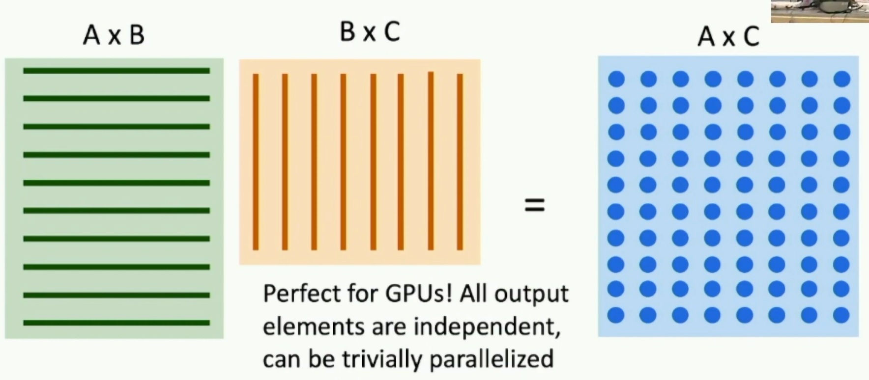
Fig: Matrix Multiplication

• Chunking the matrix into 4x4 blocks
• Powers of 2 are good for parallelism

GPU Programming

• CUDA: NVIDIA only
  • Write C code that runs directly on the GPU
  • NVIDIA provides optimized APIS: cuBLAS, cuFFT, cuDNN, etc.
• OpenCL
  • Similar to CUDA, but runs on anything
  • Usually slower on NVIDIA hardware

Scaling up: Typically 8 GPUS per server

Google Tensor Processing Units (TPU)

Cloud TPU Comparison	Performance (TFLOP/sec)	Memory	Price	Configuration
Cloud TPU v2	180 TFLOP/sec	64 GB HBM2	$4.50/hour	Single TPU
Cloud TPU v2 Pod	11.5 PFLOP/sec	-	$384/hour	64 TPU-v2
Cloud TPU v3	420 TFLOP/sec	128 GB HBM2	$8/hour	Single TPU
Cloud TPU v3 Pod	107 PFLOP/sec	-	-	256 TPU-v3

In order to use TPUs, you have to use TensorFlow (in 2019).

The most time consuming part of training a neural network is actually copying and moving data around.

Distributed Training

Model Parallelism: Different parts of the model are on different devices.

Idea 1: Run different layers of the model on different GPUs. Problem: Waiting for the slowest GPU

Idea 2: Run parallel branches of model on different GPUs. Problem: Synchronizing across GPUs

Idea 3: Batch Parallelism: Different batches of data are on different devices. GPU only communicate at the end of each batch.

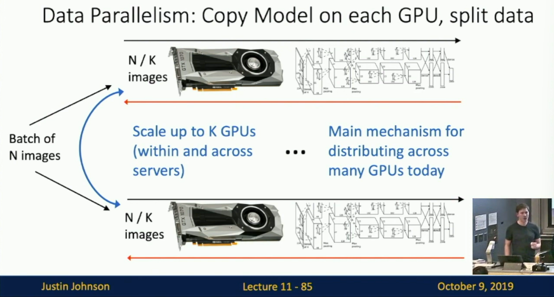
Fig: Distributed Training

Deep Learning Software

PyTorch, Caffe2, TensorFlow, PaddlePaddle, MAXNet, JAX, CNTK, Chainer, etc.

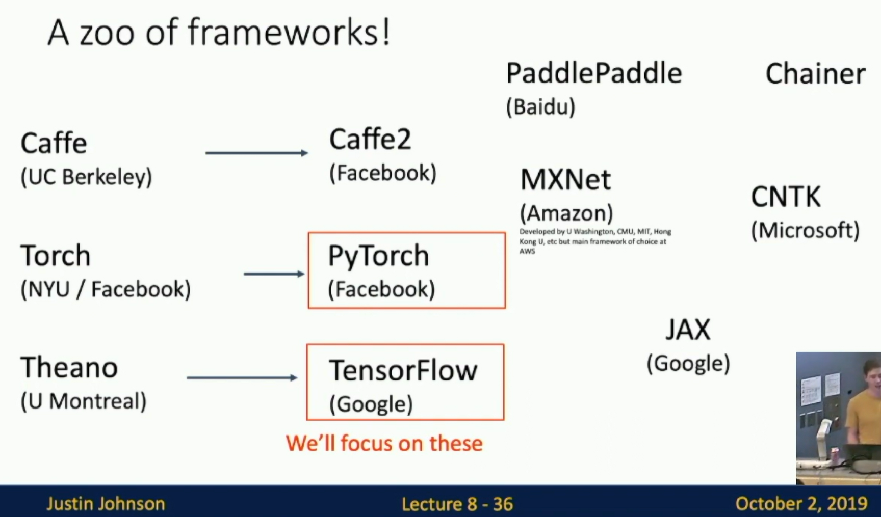
Fig: Deep Learning Software

Recall: Computational Graphs

The point of deep learning frameworks:

1. Allow rapid prototyping of new models
2. Automatically compute gradients
3. Run it all efficiently on GPUs (or TPUs)

PyTorch

Fundamental Concepts

• Tensor torch.Tensor: The basic data structure (Assignment 1, 2, 3)
• Autograd torch.autograd: Automatic differentiation
• Module torch.nn.Module: Neural network layers; may store state or learnable weights (Assignment 4, 5, 6)

Tensors

Running example: Train a two layer neural network on random data with L2 loss

# @Credits: UMich EECS 498-007 / 598-005 Deep Learning for Computer Vision
import torch

device = torch.device('cuda:0')

N, D_in, H, D_out = 64, 1000, 100, 10
x = torch.randn(N, D_in, device=device)
y = torch.randn(N, D_out, device=device)
w1 = torch.randn(D_in, H, device=device)
w2 = torch.randn(H, D_out, device=device)

learning_rate = 1e-6
for t in range(500):
    h = x.mm(w1)
    h_relu = h.clamp(min=0)
    y_pred = h_relu.mm(w2)
    loss = (y_pred - y).pow(2).sum()

    # manually compute the gradient
    grad_y_pred = 2.0 * (y_pred - y)
    grad_w2 = h_relu.t().mm(grad_y_pred)
    grad_h_relu = grad_y_pred.mm(w2.t())
    grad_h = grad_h_relu.clone()
    grad_h[h < 0] = 0
    grad_w1 = x.t().mm(grad_h)

    w1 -= learning_rate * grad_w1
    w2 -= learning_rate * grad_w2

Autograd

import torch

N, D_in, H, D_out = 64, 1000, 100, 10
x = torch.randn(N, D_in)
y = torch.randn(N, D_out)
w1 = torch.randn(D_in, H, requires_grad=True)
w2 = torch.randn(H, D_out, requires_grad=True)

learning_rate = 1e-6
for t in range(500):
    # ReLU
    y_pred = x.mm(w1).clamp(min=0).mm(w2)
    # sigmoid activation
    y_pred = sigmoid(x.mm(w1)).mm(w2)

    # The computational graph is automatically constructed
    # Clamp的意思是将小于0的值变为0
    loss = (y_pred - y).pow(2).sum()

    loss.backward()
    # Pytorch searches any leaf nodes in the computational graph
    # and computes the gradient of the loss with respect to them
    # After backward finishes, gradients are stored in the .grad
    # attribute of each tensor and the graph is **destroyed**
    with torch.no_grad():
        w1 -= learning_rate * w1.grad
        w2 -= learning_rate * w2.grad
        w1.grad.zero_()
        w2.grad.zero_()

Implement a new function

class Sigmoid(torch.autograd.Function):
    @staticmethod
    def forward(ctx, x):
        y = 1.0 / (1.0 + (-x).exp())
        ctx.save_for_backward(y)
        return y

    @staticmethod
    def backward(ctx, grad_y):
        y, = ctx.saved_tensors
        grad_x = grad_y * y * (1.0 - y)
        return grad_x

def sigmoid(x):
    return Sigmoid.apply(x)

In practice this is rare.

Module: nn

import torch

N, D_in, H, D_out = 64, 1000, 100, 10
x = torch.randn(N, D_in)
y = torch.randn(N, D_out)

model = torch.nn.Sequential(
    torch.nn.Linear(D_in, H),
    torch.nn.ReLU(),
    torch.nn.Linear(H, D_out)
)

learning_rate = 1e-2
for t in range(500):
    y_pred = model(x)
    loss = torch.nn.functional.mse_loss(y_pred, y)
    
    loss.backward()
    
    with torch.no_grad():
        for param in model.parameters():
            param -= learning_rate * param.grad
    model.zero_grad()

Optim

import torch

N, D_in, H, D_out = 64, 1000, 100, 10
x = torch.randn(N, D_in)
y = torch.randn(N, D_out)

model = torch.nn.Sequential(
    torch.nn.Linear(D_in, H),
    torch.nn.ReLU(),
    torch.nn.Linear(H, D_out)
)

learning_rate = 1e-4
optimizer = torch.optim.Adam(model.parameters(), lr=learning_rate)

for t in range(500):
    y_pred = model(x)
    loss = torch.nn.functional.mse_loss(y_pred, y)
    
    optimizer.zero_grad()
    loss.backward()
    optimizer.step()

Define your own modules

import torch

class TwoLayerNet(torch.nn.Module):
    def __init__(self, D_in, H, D_out):
        super(TwoLayerNet, self).__init__()
        self.linear1 = torch.nn.Linear(D_in, H)
        self.linear2 = torch.nn.Linear(H, D_out)

    def forward(self, x):
        h_relu = self.linear1(x).clamp(min=0)
        y_pred = self.linear2(h_relu)
        return y_pred

N, D_in, H, D_out = 64, 1000, 100, 10
x = torch.randn(N, D_in)
y = torch.randn(N, D_out)

model = TwoLayerNet(D_in, H, D_out)

optimizer = torch.optim.SGD(model.parameters(), lr=1e-4)
for t in range(500):
    y_pred = model(x)
    loss = torch.nn.functional.mse_loss(y_pred, y)

    loss.backward()
    optimizer.step()
    optimizer.zero_grad()

Example 2: ParallelBlock

import torch

class ParallelBlock(torch.nn.Module):
    def __init__(self, D_in, D_out):
        super(ParallelBlock, self).__init__()
        self.linear1 = torch.nn.Linear(D_in, D_out)
        self.linear2 = torch.nn.Linear(D_in, D_out)

    def forward(self, x):
        h1 = self.linear1(x)
        h2 = self.linear2(x)
        return (h1*h2).clamp(min=0)

N, D_in, H, D_out = 64, 1000, 100, 10
x = torch.randn(N, D_in)
y = torch.randn(N, D_out)

model = torch.nn.Sequential(
    ParallelBlock(D_in, H),
    ParallelBlock(H, H),
    torch.nn.Linear(H, D_out)
)

optimizer = torch.optim.Adam(model.parameters(), lr=1e-4)

for t in range(500):
    y_pred = model(x)
    loss = torch.nn.functional.mse_loss(y_pred, y)

    optimizer.zero_grad()
    loss.backward()
    optimizer.step()

DataLoaders

import torch
from torch.utils.data import DataLoader, TensorDataset

N, D_in, H, D_out = 64, 1000, 100, 10
x = torch.randn(N, D_in)
y = torch.randn(N, D_out)

loader = DataLoader(TensorDataset(x, y), batch_size=8)
model = TwoLayerNet(D_in, H, D_out)

optimizer = torch.optim.SGD(model.parameters(), lr=1e-4)

for epoch in range(10):
    for x_batch, y_batch in loader:
        y_pred = model(x_batch)
        loss = torch.nn.functional.mse_loss(y_pred, y_batch)

        optimizer.zero_grad()
        loss.backward()
        optimizer.step()

Pretrained Models

import torch
import torchvision

alexnet = torchvision.models.alexnet(pretrained=True)
vgg16 = torchvision.models.vgg16(pretrained=True)
resnet101 = torchvision.models.resnet101(pretrained=True)

Dynamic Computation Graphs

Dynamic graphs let you use regular Python control flow during the forward pass! This is much more flexible than static graphs.

import torch

N, D_in, H, D_out = 64, 1000, 100, 10
x = torch.randn(N, D_in)
y = torch.randn(N, D_out)
w1 = torch.randn(D_in, H, requires_grad=True)
w2a = torch.randn(H, D_out, requires_grad=True)
w2b = torch.randn(H, D_out, requires_grad=True)

learning_rate = 1e-6
prev_loss = 5.0

for t in range(500):
    w2 = w2a if prev_loss < 5.0 else w2b
    y_pred = x.mm(w1).clamp(min=0).mm(w2)
    loss = (y_pred - y).pow(2).sum()
    
    loss.backward()
    prev_loss = loss.item()

Static Graphs with JIT

@torch.jit.script
def model(x, y, w1, w2a, w2b, prev_loss):
    w2 = w2a if prev_loss < 5.0 else w2b
    y_pred = x.mm(w1).clamp(min=0).mm(w2)
    loss = (y_pred - y).pow(2).sum()
    return loss

Static:

• Once graph is built, we can serialize it and run it without the code that built the graph.
• Lots of indirection between the code you write and the code that runs - can be hard to debug, benchmark, etc.

Dynamic:

• Graph building and execution are intertwined.
• Easier to debug, benchmark, etc.
• Easily implement Recurrent and Recursive networks and other dynamic models.
• Modular Networks: You can train a network to build another network.

TensorFlow is 2.18 (Oct 2024) is moving towards a more dynamic model. Keras is the high level API for TensorFlow.

import tensorflow as tf
from tensorflow.keras.models import Sequential
from tensorflow.keras.layers import InputLayer, Dense

N, Din, H, Dout = 16, 1000, 100, 10

model = Sequential()
model.add(InputLayer(input_shape=(Din,)))
model.add(Dense(units=H, activation='relu'))
model.add(Dense(units=Dout))

params = model.trainable_variables

loss_fn = tf.keras.losses.MeanSquaredError()
opt = tf.keras.optimizers.SGD(learning_rate=1e-6)

x = tf.random.normal((N, Din))
y = tf.random.normal((N, Dout))

def step():
    y_pred = model(x)
    loss = loss_fn(y_pred, y)
    return loss

for t in range(1000):
    opt.minimize(step, params)

Tensorboard

Tensorboard is a visualization tool that comes with TensorFlow. It can be used with PyTorch as well.

import torch
import torch.utils.tensorboard

Notice on Usage and Attribution

This note is based on the University of Michigan's publicly available course EECS 498.008 / 598.008 and is intended solely for personal learning and academic discussion, with no commercial use.

• Nature of the Notes: These notes include extensive references and citations from course materials to ensure clarity and completeness. However, they are presented as personal interpretations and summaries, not as substitutes for the original course content.
• Original Course Resources: Please refer to the official University of Michigan website for complete and accurate course materials.
• Third-Party Open Access Content: This note may reference Open Access (OA) papers or resources cited within the course materials. These materials are used under their original Open Access licenses (e.g., CC BY, CC BY-SA).
• Proper Attribution: Every referenced OA resource is appropriately cited, including the author, publication title, source link, and license type.
• Copyright Notice: All rights to third-party content remain with their respective authors or publishers.
• Content Removal: If you believe any content infringes on your copyright, please contact me, and I will promptly remove the content in question.

Thanks to the University of Michigan and the contributors to the course for their openness and dedication to accessible education.