A general introduction to reinforcement learning and its applications in deep neural networks.

@Credits: EECS 498.007 | Video Lecture: UM-CV

Personal work for the assignments of the course: github repo.

Notice on Usage and Attribution

These are personal class notes based on the University of Michigan EECS 498.008 / 598.008 course. They are intended solely for personal learning and academic discussion, with no commercial use.

For detailed information, please refer to the complete notice at the end of this document

Paradigm of RL

Terms: Environment - Agent - State - Action - Reward

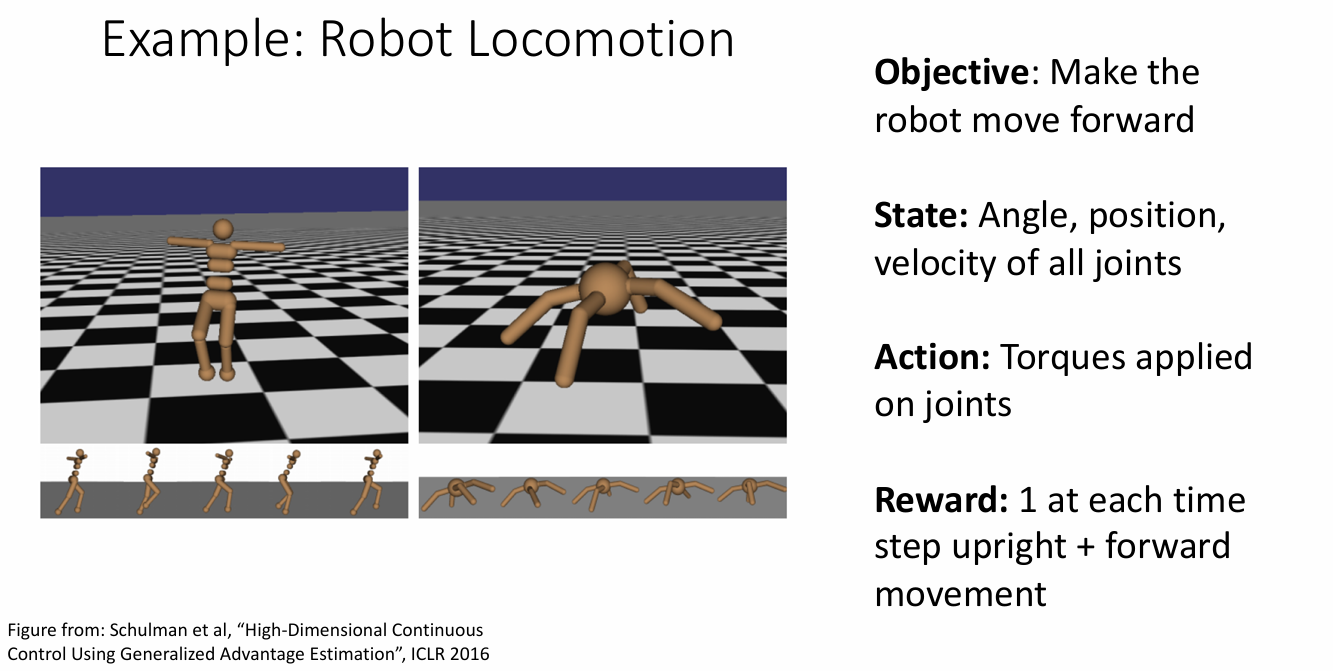
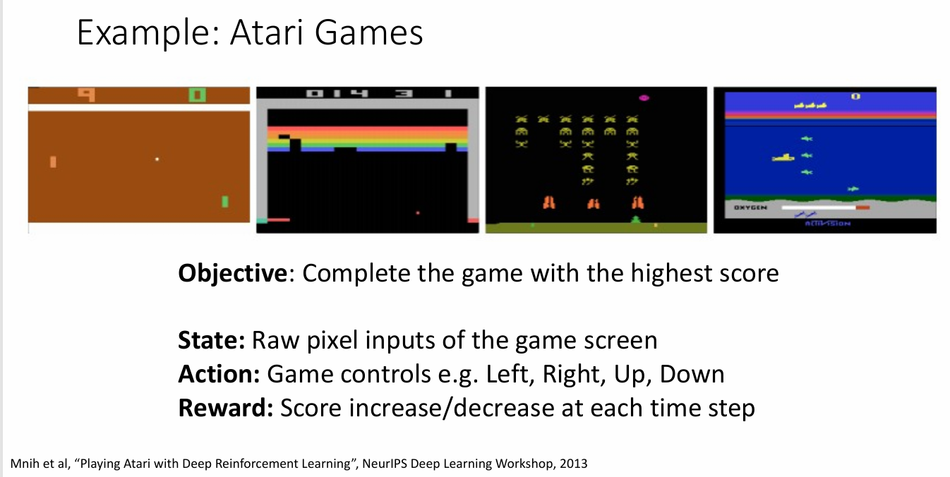
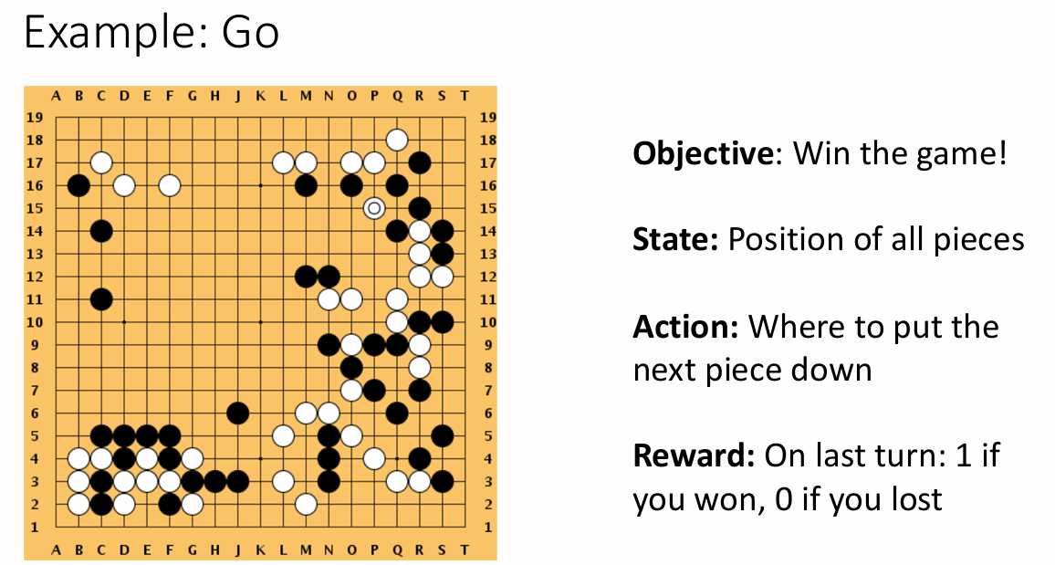
Examples

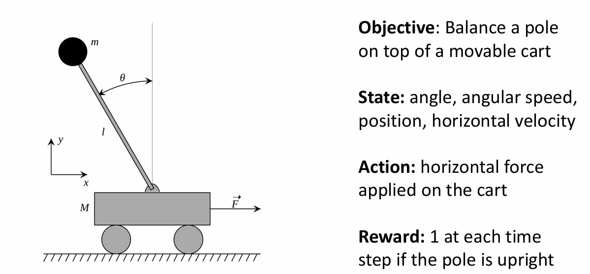
1. Cart-Pole Problem

2. Robot Locomotion

3. Atari Games

4. Go

Reinforcement Learning vs Supervised Learning

Why is RL different from normal supervised learning?

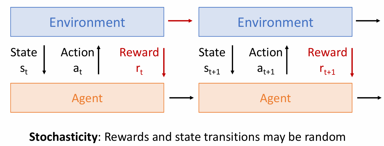
1. State transitions may be random in RL, while in supervised learning, we always apply the gradient descent to lower the loss
2. Reward $r_t$ may not directly depend on action $a_t$.
3. Non-differentiable: can't backprop through world; can't compute ${dr_t}/{da_t}$
4. Non-stationary: What the agent experiences depends on how it acts: the environment (distribution of data) changes.

Fundamentally more challenging than any supervised learning approach!

Markov Decision Process (MDP)

Mathematical formulation: A tuple $(S,A,R,P,\gamma)$

• $S$ Set of possible states
• $A$ Set of possible actions
• $R$ Distribution of reward given (state, action) pair
• $P$ Transition probability: distribution over next state given (state, action)
• $\gamma$ Discount factor (tradeoff between future and present rewards)

with respect to the Markov Property

Agent executes a policy $\pi$ giving distribution of actions conditioned on states.

Goal Find policy $\pi^*$ that maximizes cumulative discounted reward $\sum_t \gamma^t r_t$

• At time step $t=0$, environment samples initial state $s_0\sim p(s_0)$
• Then, for $t=0$ until done:
  • Agent selects action $a_t\sim\pi(a|s_t)$
  • Environment samples reward $r_t\sim R(r|s_t, a_t)$
  • Environment samples next state $s_{t+1}\sim P(s|s_t,a_t)$
  • Agent receives reward $r_t$ and next state $s_{t+1}$

Finding Optimal Policies

Goal Find the optimal policy $\pi^*$ that maximizes (discounted) sum of rewards.

Problem Lots of randomness! Initial state, transition probabilities, rewards.

Solution Maximize the expected sum of rewards

$$\pi^* = \underset{\pi}{\arg\max}\phantom{e}\mathbb{E}\left[\sum_t \gamma^t r_t|\pi\right]$$

$$s_0\sim p(s_0)\quad a_t \sim \pi(a|s_t) \quad s_{t+1} \sim P(s|s_t, a_t)$$

Value Function and Q Function

Following a policy $\pi$ produces sample trajectories (or paths)

$$s_0, a_0, r_0, s_1, a_1, r_0, ...$$

How good is a state? The value function at state $s$, is the expected cumulative reward from following policy from state $s$:

$$V^{\pi}(s) =\mathbb{E}\left[\sum_{t\geq 0}\gamma^t r_t|s_0=s,\pi\right]$$

How good is a state-action pair? The Q function at state $s$ and action $a$, is the expected cumulative reward from taking action $a$ in state $s$ and then following the policy:

$$Q^\pi(s,a)=\mathbb{E}\left[\sum_{t\geq 0}\gamma^t r_t|s_0=s,a_0=a,\pi\right]$$

By the law of total probability, we can express the value function in terms of the Q function:

$$V^\pi(s)=\sum_a \pi(a|s)Q^\pi(s,a)$$

Optimal Q-function: $Q^*$ is the Q-function for the optimal policy $\pi^*$

$$Q*(s,a)=\max_\pi Q^\pi(s,a)$$

$Q*$ encodes the optimal policy $\pi^*(s)=\arg\max_{a'}Q(s,a')$

Bellman Equation

$Q*$ satisfies the following recurrence relation:

$$Q^*(s,a)=\mathbb{E}_{r,s'}\left[r+\gamma\max_{a'}Q^*(s',a')\right]$$

where $r\sim R(r|s,a)$ and $s'\sim P(s|s,a)$.

Idea: If we find a function $Q$ that satisfies the Bellman equation, then it must be $Q^*$. Start with a random $Q$ and iteratively update it to satisfy the Bellman equation.

$$Q_{k+1}(s,a)=\mathbb{E}_{r,s'}\left[r+\gamma\max_{a'}Q_k(s',a')\right]$$

where $r\sim R(r|s,a)$ and $s'\sim P(s|s,a)$.

Amazing fact: This iterative process converges to $Q^*$!

Problem: Need to keep track of $Q(s,a)$ for every state-action pair - impossible if infinite.

Solution: Use a function approximator (e.g., neural network) to estimate $Q(s,a)$, use Bellman equation as the loss function.

Algorithms for reinforcement learning

Deep Q-Learning

Train a neural network to predict approximate $Q^*(s,a) \sim Q(s,a;\theta)$.

Use the bellman equation to tell what Q should output for a given state and action:

$$y_{s,a,\theta}=\mathbb{E}_{r,s'}\left[r+\gamma\max_{a'}Q(s',a';\theta)\right]$$

where $r\sim R(r|s,a)$ and $s'\sim P(s|s,a)$.

Then, minimize the loss for training $Q$:

$$L(s,a)=\left(y_{s,a,\theta}-Q(s,a;\theta)\right)^2$$

Problem: Nonstationary! The target for $Q(s,a)$ depends on the current weights $\theta$! Problem: How to sample batches of data for training?

For some problems this can be a hard function to learn. For some problems it is easier to learn the value function.

Policy Gradients

Directly optimize the policy $\pi(a|s;\theta)$ to maximize expected reward.

Train a network $\pi(a|s;\theta)$ to output a distribution over actions taking state $s$ as input.

Objective function: Expected reward under policy $\pi$:

$$J(\theta)=\mathbb{E}_{\tau\sim\pi}\left[\sum_{t\geq 0}\gamma^t r_t\right]$$

Find the optimal policy by gradient ascent: $\theta\leftarrow\theta+\alpha\nabla_\theta J(\theta)$

$\theta^* = \arg\max_\theta J(\theta)$

Problem: Non-differentiable! How to compute $\nabla_\theta J(\theta)$?

General idea: $J(\theta)=\mathbb{E}_{x\sim p_\theta(x)}[f(x)]$ Want to compute $\nabla_\theta J(\theta)$

$$\nabla_\theta J(\theta)=\mathbb{E}_{x\sim p_\theta(x)}[f(x)\nabla_\theta\log p_\theta(x)]$$

Approximate via sampling!

REINFORCE Algorithm

1. Collect a trajectory $\tau=(s_0,a_0,r_0,s_1,a_1,r_1,...)$ by following policy $\pi_\theta$. It's ramdom: $x\sim p_\theta(x)$

$$p_\theta(x) = \prod_{t\geq 0} P(s_{t+1}|s_t)\pi_\theta(a_t|s_t) \\ \implies \log p_\theta(x) = \sum_{t\geq 0}\log P(s_{t+1}|s_t)+\log\pi_\theta(a_t|s_t) \\ \implies \nabla_\theta\log p_\theta(x) = \sum_{t\geq 0}\nabla_\theta\log\pi_\theta(a_t|s_t)$$

Expected reward under $\pi_\theta$:

$$J(\theta)=\mathbb{E}_{x\sim p_\theta(x)}[f(x)]$$

$$\nabla_\theta J(\theta)=\mathbb{E}_{x\sim p_\theta(x)}[f(x)\nabla_\theta\log p_\theta(x)]$$

1. Initialize random weights $\theta$
2. Collect trajectories $x$ and rewards $f(x)$ using policy $\pi_\theta$
3. Compute $\nabla_\theta J(\theta)$ using samples
4. gradient ascent: $\theta\leftarrow\theta+\alpha\nabla_\theta J(\theta)$
5. Goto 2

Intuition: when $f(x)$ is high, increase the probability of the actions we took. When $f(x)$ is low, decrease the probability of the actions we took.

Recap

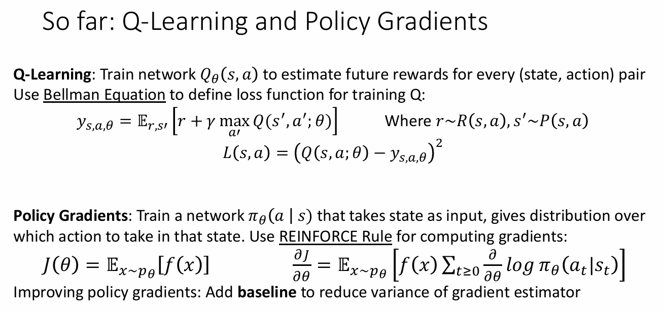
Other approaches: Model based RL

Actor-Critic, Trust Region Policy Optimization, Proximal Policy Optimization, etc.

Actor Critic: Train an actor that predicts actions (like policy gradients) and a critics that predicts value functions (like Q-learning).

Model-based: Learn a model of the world's state transition function and then use planning to find the optimal policy.

Inverse Reinforcement Learning: Gather data of experts performing in environment; learn a reward function that they seem to be optimizing, then use RL on that reward function.

Adversarial Learning: Learn to fool a discriminator that tries to distinguish between real and fake trajectories.

Examples

1. AlphaGo (2016): Policy network (actor) and value network (critic) trained with policy gradients.
2. AlphaGO Zero (2017): Reinforcement learning with self-play and Monte Carlo Tree Search.
3. Alpha Zero (2018): Generalized to other games: Chess and Shogi
4. MuZero (2019): Plans through a learned model of the game.
5. OpenAI Five (Apr 2019): Proximal Policy Optimization (PPO) with a model-based RL component.

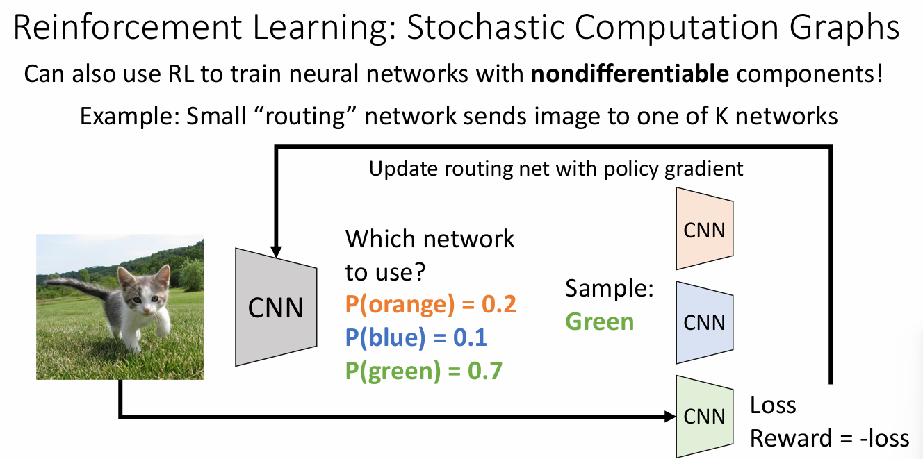
Stochastic Computation Graphs

Notice on Usage and Attribution

This note is based on the University of Michigan's publicly available course EECS 498.008 / 598.008 and is intended solely for personal learning and academic discussion.

• Nature of the Notes: These notes include extensive references and citations from course materials to ensure clarity and completeness. However, they are presented as personal interpretations and summaries, not as substitutes for the original course content. Please refer to the official University of Michigan website for complete and accurate course materials.
• Third-Party Open Access Content: This note may reference Open Access (OA) papers or resources cited within the course materials. These materials are used under their original Open Access licenses (e.g., CC BY, CC BY-SA). Every referenced OA resource is appropriately cited, including the author, publication title, source link, and license type.
• Copyright: All rights to third-party content remain with their respective authors or publishers. If you believe any content infringes on your copyright, please contact me, and I will promptly remove the content in question.

Thanks to the University of Michigan and the contributors to the course for their openness and dedication to accessible education.