Summary:

Part 1: Neural Networks, Activation Functions, Biological Neurons, Space Warping, Universal Approximation, Convergence of Neural Networks

Part 2: Backpropagation, Computational graphs, Modular implementation, automatic differentiation, Higher-order derivatives

@Credits: EECS 498.007 | Video Lecture: UM-CV

Personal work for the assignments of the course: github repo.

Notice on Usage and Attribution

These are personal class notes based on the University of Michigan EECS 498.008 / 598.008 course. They are intended solely for personal learning and academic discussion, with no commercial use.

For detailed information, please refer to the complete notice at the end of this document

Neural Networks

Linear classifiers are limited to their linear decision boundaries. Neural networks are more flexible and can learn more complex decision boundaries.

Feature extraction

Color histograms, HOG, SIFT, etc. (2000-2010)

• Color histograms - Statistical Method
• HOG: Histogram of Oriented Gradients
  • Compute edge direction/strength at each pixel
• Bag of Words(Data-Driven) - Clustering
  1. Extract random patches from images &Cluster patches into "codebook" of visual words
  2. Encode each image as histogram of visual words
• Concatenate features together - Different methods can capture different features of the image

2011 ImageNet Winner: A complicated feature extractor

SIFT: Scale-Invariant Feature Transform 128-D vector

color: 96-D vector

Reduced to 64-D with PCA

FV extraction and compression

One-vs-all SVM learning with SGD

Late fusion of SIFT and color systems

Problem: These complicated systems are not designed to directly minimize the classification error!

AlexNet: Deep Learning (2012)

Deep Neural Networks (DNNs) are end-to-end trainable!

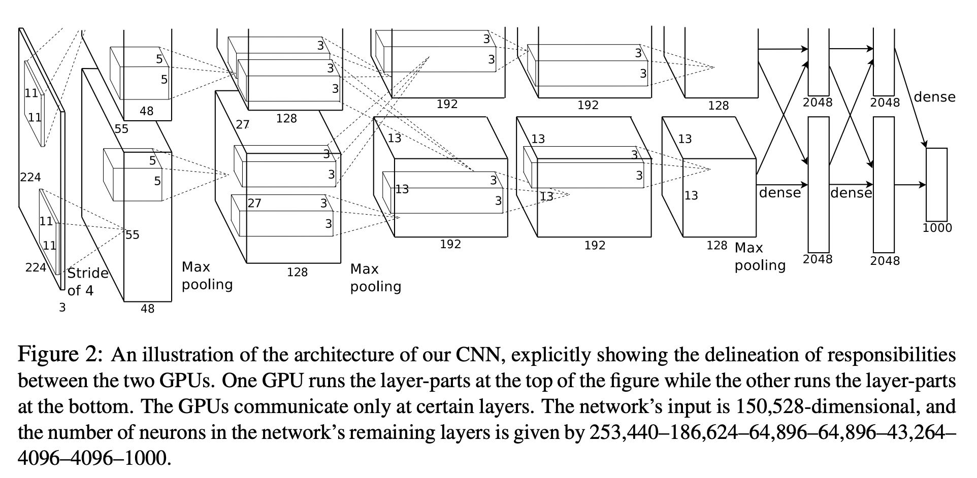
Fig: AlexNet

Neural Networks

(Before) Linear score function: $f(x, W) = Wx$

(Now) 2-layer Neural Network: $f(x, W) = W_2\max(0, W_1x)$

where $x\in\mathbb{R}^D$,$W_1\in\mathbb{R}^{H\times D}$, $W_2\in\mathbb{R}^{C\times H}$

or 3-layer Neural Network

$$f(x, W) = W_3\max(0, W_2\max(0, W_1x))$$

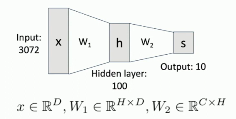
Fig: Data Flow

Deep Neural Networks

Each output is affected by each input: Fully connected network (or MLP - Multi-Layer Perceptron), and templates (each row of the matrix $W$) are combined layerwise.

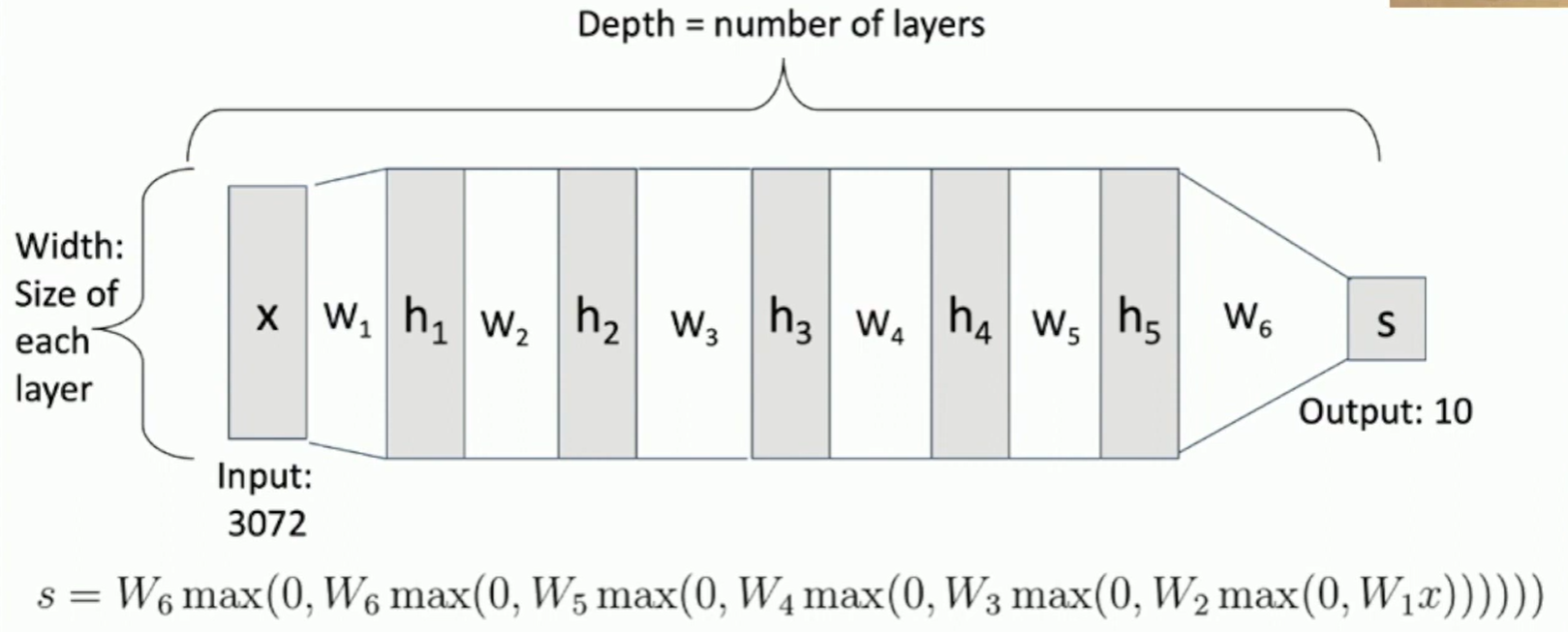
Fig: DNN

Activation Functions

Add non-linearity to the network. Without non-linearity, the network would be equivalent to a single layer.

The most widely used: ReLU (Rectified Linear Unit)

$$\text{ReLu}(x) = \max(0, x)$$

Sigmoid

$$\sigma(x) = \frac{1}{1+e^{-x}}$$

Tanh

$$\tanh(x) = \frac{e^x - e^{-x}}{e^x + e^{-x}}$$

Leaky ReLU

$$\text{Leaky ReLU}(x) = \max(0.01x, x)$$

Maxout

$$\text{Maxout}(x) = \max(w_1^Tx + b_1, w_2^Tx + b_2)$$

ELU

$$\text{ELU}(x) = \begin{cases} x & \text{if } x > 0 \\ \alpha(e^x - 1) & \text{if } x \leq 0 \end{cases}$$

Neural Network in < 20 lines!

import numpy as np
from numpy.random import randn
N, Din, H, Dout, = 64, 1000, 100, 10
x, y = randn(N, Din), randn(N, Dout)
w1, w2 = randn(Din, H), randn(H, Dout)
learning_rate = 1e-6
for t in range(10000):
  h = 1/(1 + np.exp(-x.dot(w1)))
  y_pred = h.dot(w2)
  loss = np.square(y_pred - y).sum()
  grad_y_pred = 2.0 * (y_pred - y)
  grad_w2 = h.T.dot(grad_y_pred)
  grad_h = grad_y_pred.dot(w2.T)
  grad_w1 = x.T.dot(grad_h * h * (1 - h))
  w1 -= learning_rate * grad_w1
  w2 -= learning_rate * grad_w2

Analogy: Biological Neurons

Our brains are made of neurons. Impulses are carried away from cell body. Dendrites receive impulses from other neurons. Synapses are connections between neurons.

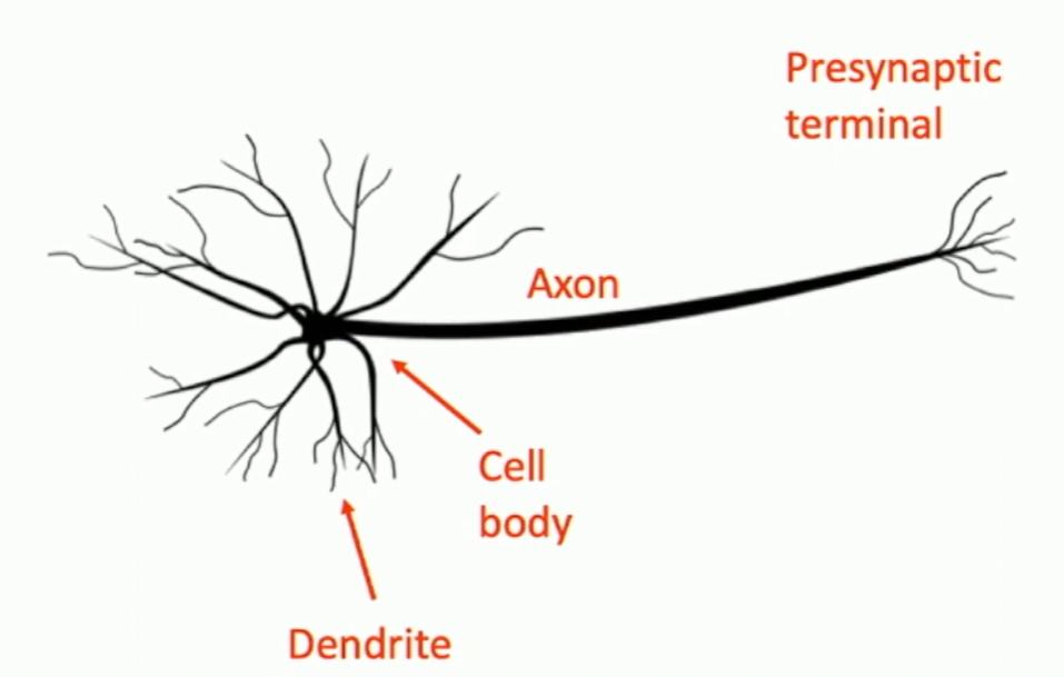
Fig: Biological Neurons

Differences between biological and artificial neurons

• Biological neurons have complex connectivity patterns
• Inside a neuron, signals are computed by complex processes
• Artificial neurons are organized into regular layers for computational efficiency

Fun fact: But neural networks with random connectivity can still learn!

Space Warping

A linear layer cannot improve the representation power of the classifier, but with a non-linear transform in between, the classifier can learn more complex decision boundaries.

Explanation: Space Warping

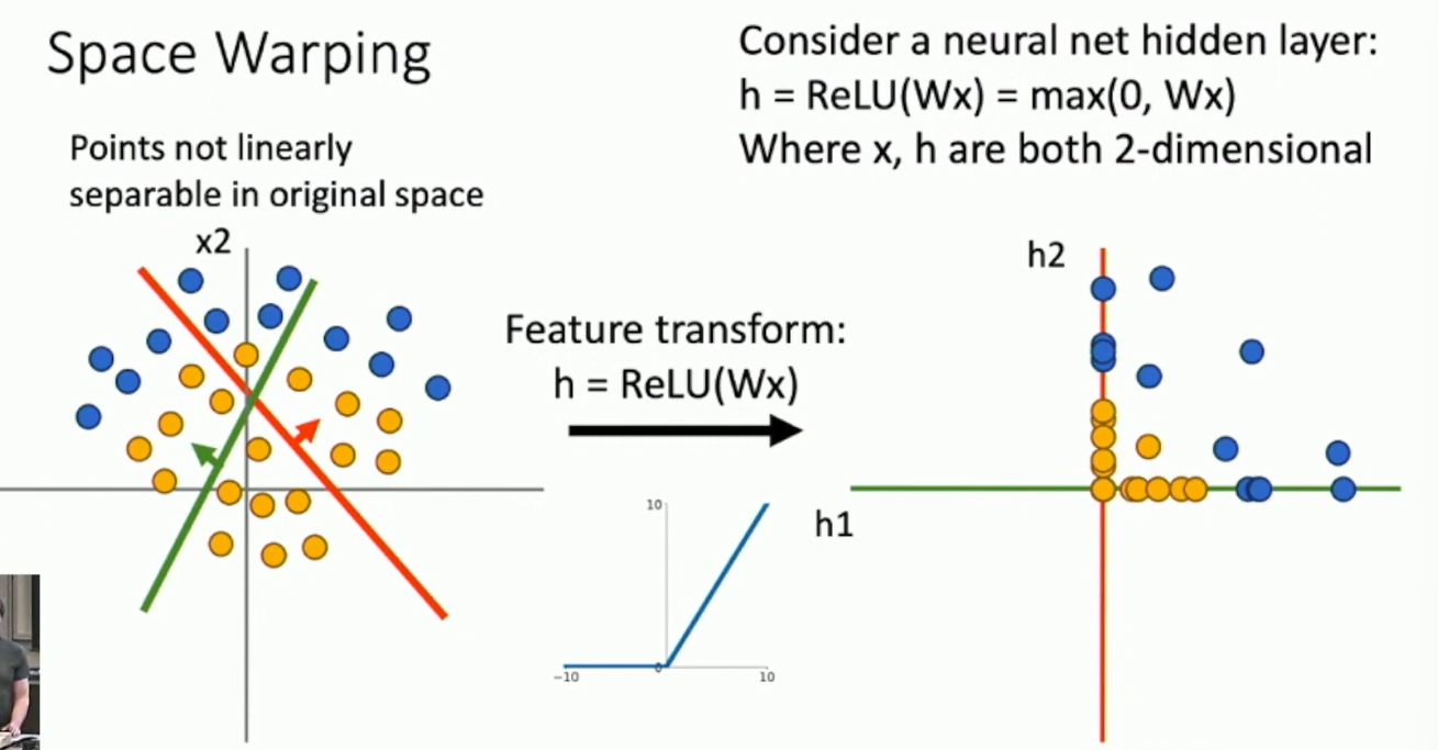
Fig: Space Warping

Points can be linearly separable in a higher-dimensional space.

Technique: Don't regularize with size; instead use stronger L2.

Universal Approximation

A neural network with a single hidden layer can approximate any continuous function to arbitrary accuracy (uniformly convergent), on compacts of $\mathbb{R}^n$.

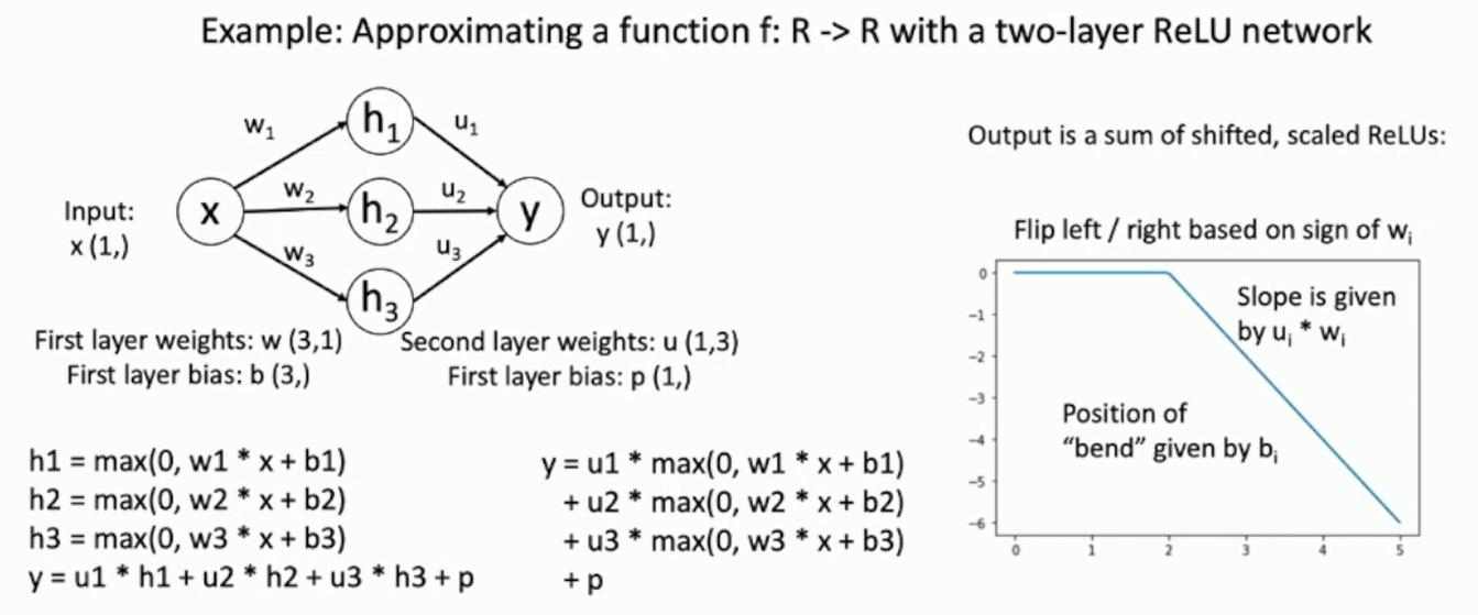
Fig: Universal Approximation

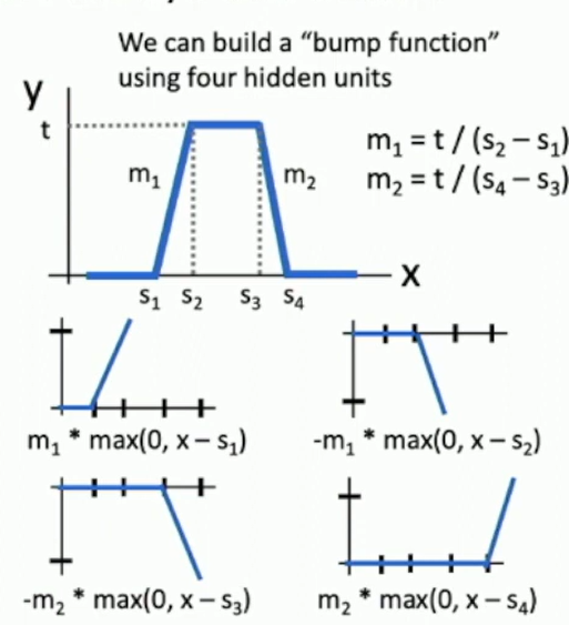
Fig: Bump function as basis

See Nielsen's Neural Networks and Deep Learning for more details.

Reality check: Networks don't really learn bumps!

But the theorem does not tell us how to find the right weights, given that $f$ is unknown a priori.

Convergence of Neural Networks

Definition: (Convexity) A function $f: \mathbb{R}^D \to \mathbb{R}$ is convex if for all $x, y \in \mathbb{R}^D$ and $t \in [0, 1]$, we have

$$f(t x + (1 - t)y) \leq t f(x) + (1 - t)f(y)$$

Theorem: A single layer neural network with ReLU activation is a convex function of its weights.

No such guarantee for non-linear networks.

Neural net losses sometimes look convex-ish.

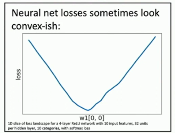
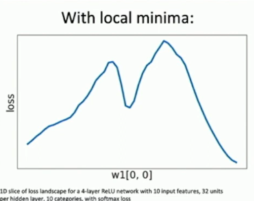
Fig: loss surfaces

Open question: theoretical properties of the optimization landscape of neural networks.

Summary of lecture 5

• Feature transform
• Neural networks
• Activation functions
• Biological neurons
• Space warping
• Universal approximation
• Convergence of neural networks

Backpropagation

Problem: How to compute the gradient of the loss function with respect to the weights?

(Bad) Idea: Derive $\frac{\partial L}{\partial W}$ by hand

See what I have done Derive gradient by hand

Computational graphs

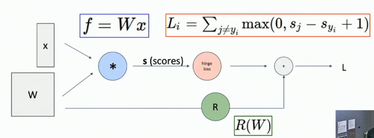
Fig: computational graph of a SVM

This is critical for large neural networks, e.g. AlexNet or Recurrent Neural Turing Machine...

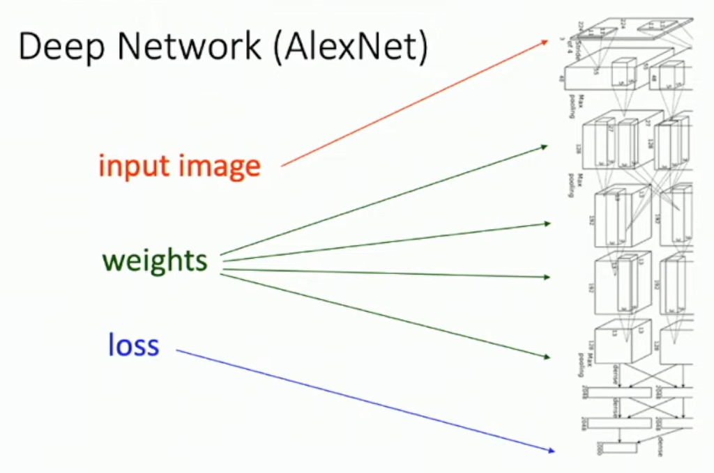
Fig: AlexNet

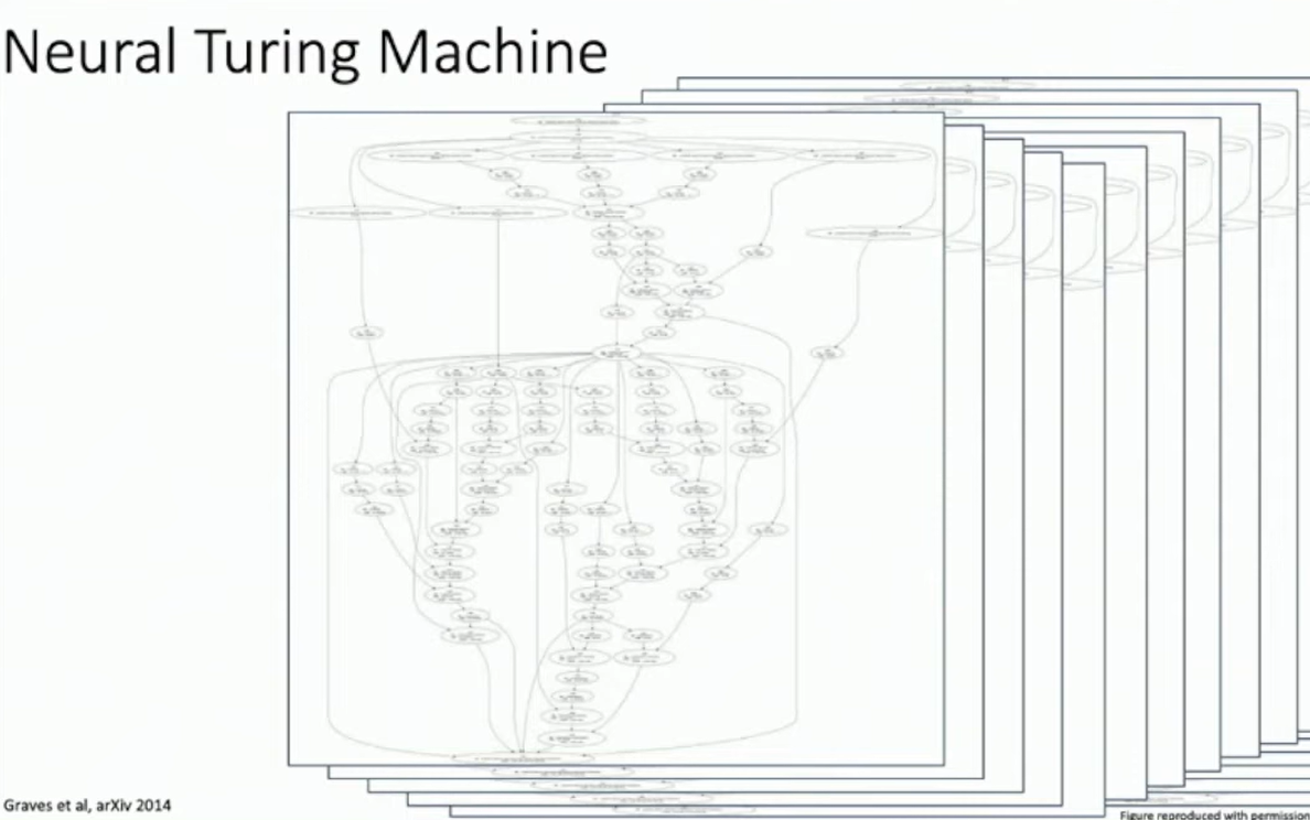
Fig: Recurrent Neural Turing Machine

Examples

Example 1

$$f(x, y, z) = (x + y)z \quad x=-2, y=5, z=-4$$

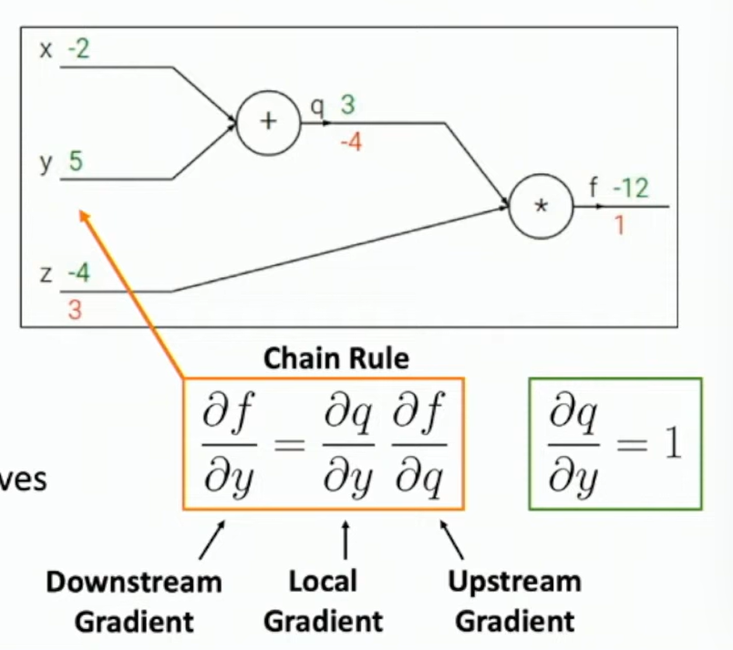
Fig: Backpropagation example 1

1. Forward pass: Compute outputs $q = x + y$ and $f = qz$
2. Backward pass: Compute gradients $\frac{\partial f}{\partial q}$ and $\frac{\partial f}{\partial z}$

$$\frac{\partial f}{\partial f} = 1 \quad \frac{\partial f}{\partial q} = z \quad \frac{\partial f}{\partial z} = q$$

$$\frac{\partial f}{\partial x} = \frac{\partial f}{\partial q} \frac{\partial q}{\partial x} = z \cdot 1 = -4$$

$$\frac{\partial f}{\partial y} = \frac{\partial f}{\partial q} \frac{\partial q}{\partial y} = z \cdot 1 = -4$$

We can compute local gradient of one node and the chain rules can be implemented as modules.

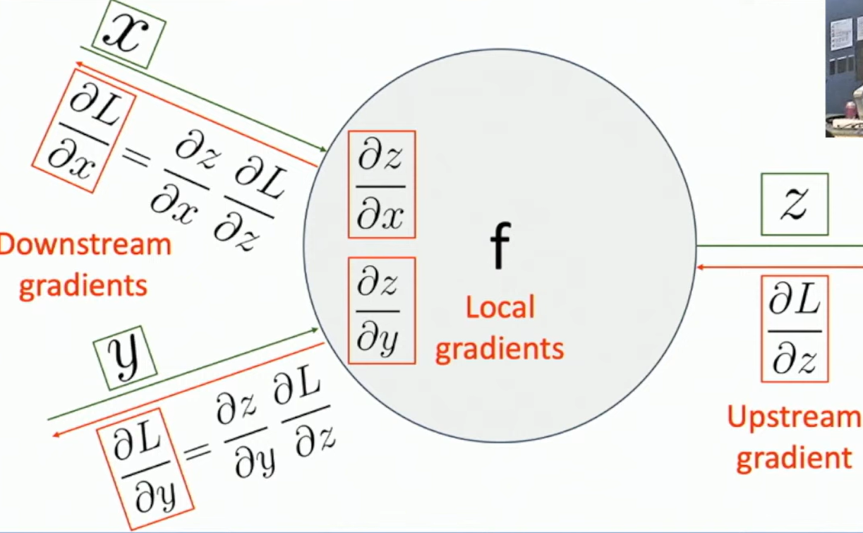
Fig: local gradient computation

Example 2

$$f(x,w) = \frac{1}{1 + e^{-(w_0x_0+w_1x_1)}}$$

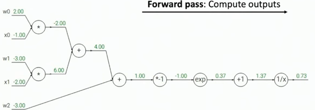
Fig: Backpropagation example 2

We can also choose more primitive functions for which the gradients are easy to compute.

e.g. Sigmoid functions

$$\sigma(x) = \frac{1}{1 + e^{-x}} \quad \frac{d\sigma}{dx} = \sigma(x)(1 - \sigma(x))$$

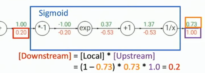
Fig: Sigmoid function

Pattern in gradient Flow

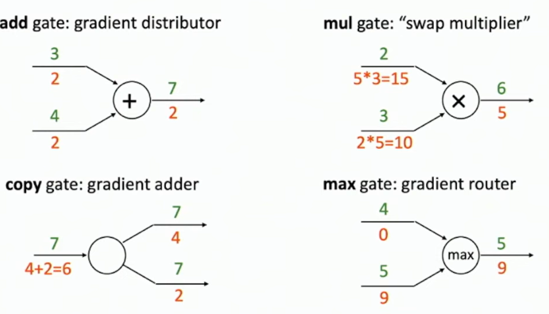
Fig: Patterns in Gradient flow

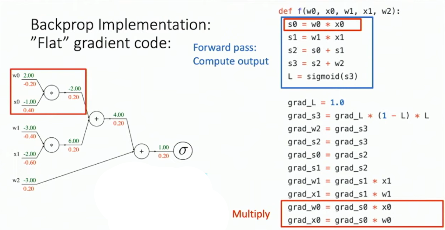
Fig: Backprop Implementation

Modular Implementation

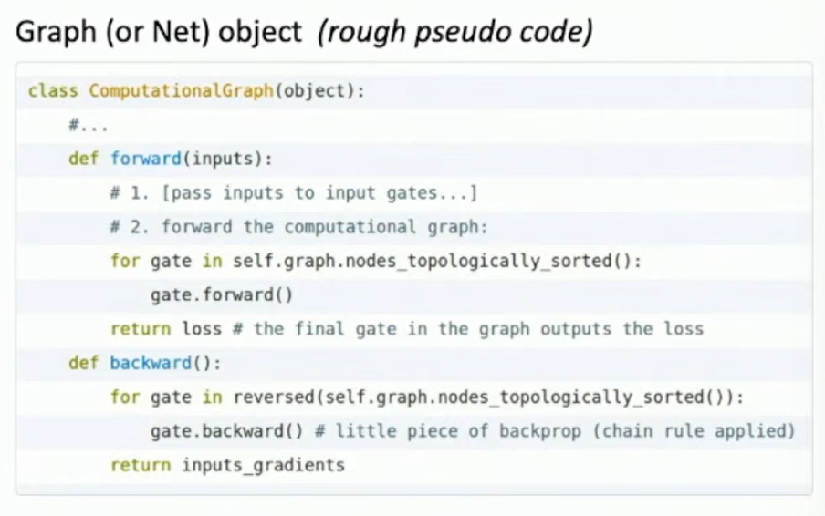
Fig: Modular Implementation

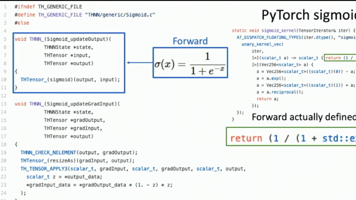
Fig: Backpropagation of Sigmoid function

Backpropagation for vector-based functions

In this course, the jacobian matrix is the transpose of that in mathematics...

$$\frac{\partial f}{\partial x} = \begin{bmatrix} \frac{\partial f_1}{\partial x_1} & \cdots & \frac{\partial f_m}{\partial x_1} \\ \vdots & \ddots & \vdots \\ \frac{\partial f_1}{\partial x_n} & \cdots & \frac{\partial f_m}{\partial x_n} \end{bmatrix}\in\mathbb{R}^{n\times m}$$

Local gradient calculation:

Let $f$ be a vector-valued function $f: \mathbb{R}^n \to \mathbb{R}^m$, and $y = f(x)$. Suppose we have calculated $\frac{\partial l}{\partial y}\in\mathbb{R}^{m}$, then

$$\underbrace{\frac{\partial l}{\partial x}}_{\text{grad\_x}} = \underbrace{\frac{\partial f}{\partial g}(x)}_{\text{local grad module}}\cdot \underbrace{\frac{\partial l}{\partial y}}_{\text{grad\_y}}(y)$$

Again we have omitted transposing $\frac{\partial l}{\partial y}$.

In practice, we never actually compute the jacobian matrix, but instead compute the product of the jacobian and a vector.

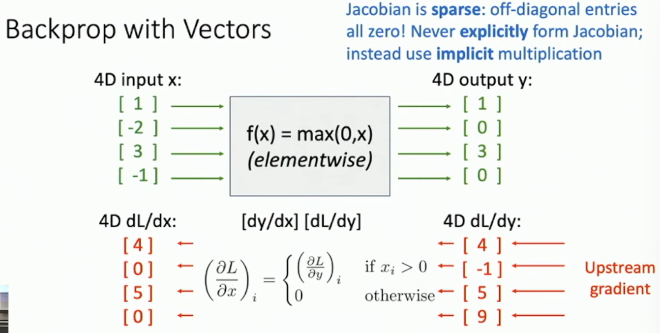
Fig: Backpropagation for vectors

Backpropagation for Matrices (or Tensors)

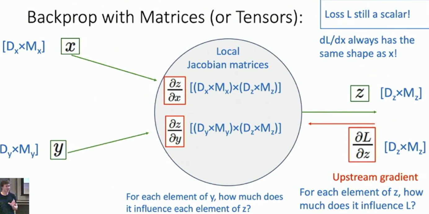
Fig: Backpropagation with Matrices

How to generalize the matrix product?

We can use the Einstein summation convention to generalize the matrix product.

Let $X\in\mathbb{R}^{m\times n}$ and a matrix function $Y=f: \mathbb{R}^{m\times n} \to \mathbb{R}^{p\times q}$. Suppose we have calculated $\frac{\partial l}{\partial Y}\in\mathbb{R}^{p\times q}$, then

$$\frac{\partial l}{\partial X} = \frac{\partial f}{\partial X}(X) \cdot \frac{\partial l}{\partial Y}$$

where $\frac{\partial f}{\partial X}(X)$ is a tensor of shape $(m, n, p, q)$.

With the Einstein summation convention, we can write this as

$$\frac{\partial l}{\partial X}_{ij} = \frac{\partial f_{kl}}{\partial X_{ij}} \frac{\partial l}{\partial Y_{kl}}$$

The trick here is to find a quick way to carry out the computation implicitly without actually constructing the jacobian tensor.

Reverse-Mode Automatic Differentiation

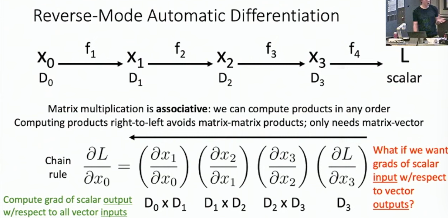
Fig: Reverse-Mode Automatic Differentiation

Forward-Mode Automatic Differentiation

This is used when the input is a scalar.

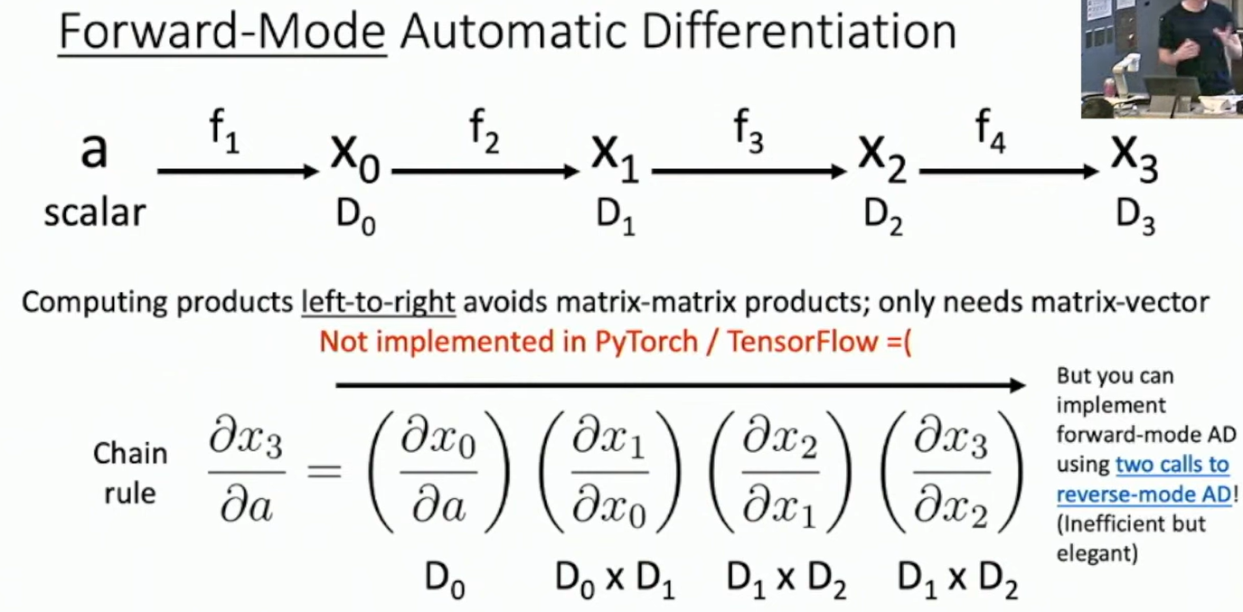
Fig: Backpropagation with Matrices

Backprop: Higher-Order Derivatives

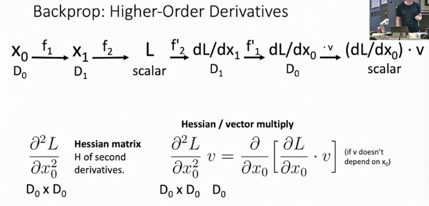
Fig: Higher-Order Derivatives

If we want to calculate the Hessian/vector product, we can construct this by hand.

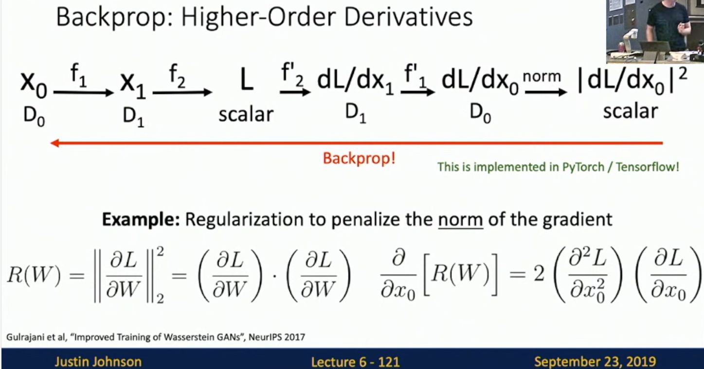
Fig: Application of Higher-Order Derivatives as a penalization

Summary of lecture 6

• Backpropagation
• Computational graphs
• Examples of backpropagation
• Gradient flow patterns
• Modular implementation
• Backpropagation for vector-based functions
• Backpropagation for matrices (or tensors)
• Reverse-mode automatic differentiation
• Forward-mode automatic differentiation
• Higher-order derivatives

Notice on Usage and Attribution

This note is based on the University of Michigan's publicly available course EECS 498.008 / 598.008 and is intended solely for personal learning and academic discussion, with no commercial use.

• Original Course Resources: Please refer to the official University of Michigan website for complete and accurate course materials.
• Third-Party Open Access Content: This note may reference Open Access (OA) papers or resources cited within the course materials. These materials are used under their original Open Access licenses (e.g., CC BY, CC BY-SA).
• Proper Attribution: Every referenced OA resource is appropriately cited, including the author, publication title, source link, and license type.
• Copyright Notice: All rights to third-party content remain with their respective authors or publishers.
• Content Removal: If you believe any content infringes on your copyright, please contact me, and I will promptly remove the content in question.

Thanks to the University of Michigan and the contributors to the course for their openness and dedication to accessible education.